Fairness and Explainability with SageMaker Clarify - Spark Distributed Processing
This notebook’s CI test result for us-west-2 is as follows. CI test results in other regions can be found at the end of the notebook.
Runtime
This notebook takes approximately 30 minutes to run.
Contents
Overview
Amazon SageMaker Clarify helps improve your machine learning models by detecting potential bias and helping explain how these models make predictions. The fairness and explainability functionality provided by SageMaker Clarify takes a step towards enabling AWS customers to build trustworthy and understandable machine learning models. The product comes with the tools to help you with the following tasks.
Measure biases that can occur during each stage of the ML lifecycle (data collection, model training and tuning, and monitoring of ML models deployed for inference).
Generate model governance reports targeting risk and compliance teams and external regulators.
Provide explanations of the data, models, and monitoring used to assess predictions.
In doing so, the notebook first trains a SageMaker XGBoost model using training dataset, then use Amazon SageMaker Python SDK to launch SageMaker Clarify jobs to analyze an example dataset in CSV format. This notebook specifically showcases how to use Spark distributed processing for executing clarify jobs.
Prerequisites and Data
Import Libraries
[2]:
from sagemaker import session, get_execution_role
from io import StringIO
from s3fs import S3FileSystem
import sagemaker
import json
import pandas as pd
import numpy as np
import seaborn as sns
import matplotlib.pyplot as plt
import os
import boto3
Set Configurations
[3]:
# Initialize sagemaker session
sagemaker_session = session.Session()

region = sagemaker_session.boto_region_name
print(f"Region: {region}")

role = get_execution_role()
print(f"Role: {role}")

bucket = sagemaker_session.default_bucket()

prefix = "sagemaker/DEMO-sagemaker-clarify"
Region: us-west-2
Role: arn:aws:iam::000000000000:role/service-role/AmazonSageMaker-ExecutionRole-20220304T121686
Download data
Data Source: https://archive.ics.uci.edu/ml/machine-learning-databases/adult/
Let’s download the data and save it in the local folder with the name adult.data and adult.test from UCI repository\(^{[2]}\).
\(^{[2]}\)Dua Dheeru, and Efi Karra Taniskidou. “UCI Machine Learning Repository”. Irvine, CA: University of California, School of Information and Computer Science (2017).
[4]:
from sagemaker.s3 import S3Downloader

adult_columns = [
    "Age",
    "Workclass",
    "fnlwgt",
    "Education",
    "Education-Num",
    "Marital Status",
    "Occupation",
    "Relationship",
    "Ethnic group",
    "Sex",
    "Capital Gain",
    "Capital Loss",
    "Hours per week",
    "Country",
    "Target",
]
if not os.path.isfile("adult.data"):
    S3Downloader.download(
        s3_uri="s3://{}/{}".format(
            f"sagemaker-example-files-prod-{region}", "datasets/tabular/uci_adult/adult.data"
        ),
        local_path="./",
        sagemaker_session=sagemaker_session,
    )
    print("adult.data saved!")
else:
    print("adult.data already on disk.")

if not os.path.isfile("adult.test"):
    S3Downloader.download(
        s3_uri="s3://{}/{}".format(
            f"sagemaker-example-files-prod-{region}", "datasets/tabular/uci_adult/adult.test"
        ),
        local_path="./",
        sagemaker_session=sagemaker_session,
    )
    print("adult.test saved!")
else:
    print("adult.test already on disk.")
adult.data saved!
adult.test saved!
Loading the data: Adult Dataset
From the UCI repository of machine learning datasets, this database contains 14 features concerning demographic characteristics of 45,222 rows (32,561 for training and 12,661 for testing). The task is to predict whether a person has a yearly income that is more or less than $50,000.
Here are the features and their possible values:
Age: continuous.
Workclass: Private, Self-emp-not-inc, Self-emp-inc, Federal-gov, Local-gov, State-gov, Without-pay, Never-worked.
Fnlwgt: continuous (the number of people the census takers believe that observation represents).
Education: Bachelors, Some-college, 11th, HS-grad, Prof-school, Assoc-acdm, Assoc-voc, 9th, 7th-8th, 12th, Masters, 1st-4th, 10th, Doctorate, 5th-6th, Preschool.
Education-num: continuous.
Marital-status: Married-civ-spouse, Divorced, Never-married, Separated, Widowed, Married-spouse-absent, Married-AF-spouse.
Occupation: Tech-support, Craft-repair, Other-service, Sales, Exec-managerial, Prof-specialty, Handlers-cleaners, Machine-op-inspct, Adm-clerical, Farming-fishing, Transport-moving, Priv-house-serv, Protective-serv, Armed-Forces.
Relationship: Wife, Own-child, Husband, Not-in-family, Other-relative, Unmarried.
Ethnic group: White, Asian-Pac-Islander, Amer-Indian-Eskimo, Other, Black.
Sex: Female, Male.
Note: this data is extracted from the 1994 Census and enforces a binary option on Sex
Capital-gain: continuous.
Capital-loss: continuous.
Hours-per-week: continuous.
Native-country: United-States, Cambodia, England, Puerto-Rico, Canada, Germany, Outlying-US(Guam-USVI-etc), India, Japan, Greece, South, China, Cuba, Iran, Honduras, Philippines, Italy, Poland, Jamaica, Vietnam, Mexico, Portugal, Ireland, France, Dominican-Republic, Laos, Ecuador, Taiwan, Haiti, Columbia, Hungary, Guatemala, Nicaragua, Scotland, Thailand, Yugoslavia, El-Salvador, Trinadad&Tobago, Peru, Hong, Holand-Netherlands.
Next, we specify our binary prediction task:
Target: <=50,000, >$50,000.
[5]:
training_data = pd.read_csv(
    "adult.data", names=adult_columns, sep=r"\s*,\s*", engine="python", na_values="?"
).dropna()

testing_data = pd.read_csv(
    "adult.test", names=adult_columns, sep=r"\s*,\s*", engine="python", na_values="?", skiprows=1
).dropna()

training_data.head()
[5]:
| Age | Workclass | fnlwgt | Education | Education-Num | Marital Status | Occupation | Relationship | Ethnic group | Sex | Capital Gain | Capital Loss | Hours per week | Country | Target | |
|---|---|---|---|---|---|---|---|---|---|---|---|---|---|---|---|
| 0 | 39 | State-gov | 77516 | Bachelors | 13 | Never-married | Adm-clerical | Not-in-family | White | Male | 2174 | 0 | 40 | United-States | <=50K |
| 1 | 50 | Self-emp-not-inc | 83311 | Bachelors | 13 | Married-civ-spouse | Exec-managerial | Husband | White | Male | 0 | 0 | 13 | United-States | <=50K |
| 2 | 38 | Private | 215646 | HS-grad | 9 | Divorced | Handlers-cleaners | Not-in-family | White | Male | 0 | 0 | 40 | United-States | <=50K |
| 3 | 53 | Private | 234721 | 11th | 7 | Married-civ-spouse | Handlers-cleaners | Husband | Black | Male | 0 | 0 | 40 | United-States | <=50K |
| 4 | 28 | Private | 338409 | Bachelors | 13 | Married-civ-spouse | Prof-specialty | Wife | Black | Female | 0 | 0 | 40 | Cuba | <=50K |
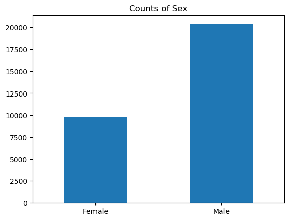
Data inspection
[6]:
%matplotlib inline
training_data["Sex"].value_counts().sort_values().plot(kind="bar", title="Counts of Sex", rot=0)
[6]:
<matplotlib.axes._subplots.AxesSubplot at 0x7f051c2362d0>
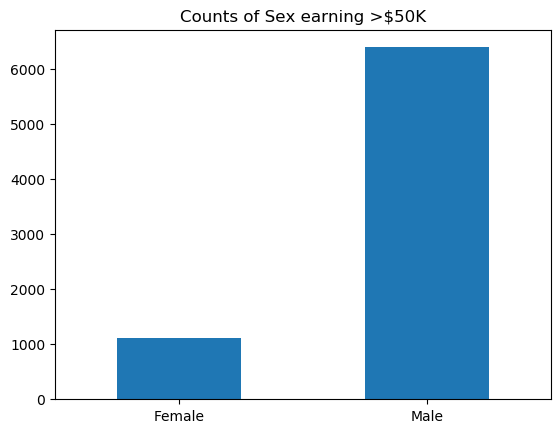
[7]:
training_data["Sex"].where(training_data["Target"] == ">50K").value_counts().sort_values().plot(
    kind="bar", title="Counts of Sex earning >$50K", rot=0
)
[7]:
<matplotlib.axes._subplots.AxesSubplot at 0x7f051c242990>
Encode and Upload the Dataset
Here we encode the training and test data. Encoding input data is not necessary for SageMaker Clarify, but is necessary for the model.
[8]:
from sklearn import preprocessing


def number_encode_features(df):
    result = df.copy()
    encoders = {}
    for column in result.columns:
        if result.dtypes[column] == np.object:
            encoders[column] = preprocessing.LabelEncoder()
            #  print('Column:', column, result[column])
            result[column] = encoders[column].fit_transform(result[column].fillna("None"))
    return result, encoders


training_data = pd.concat([training_data["Target"], training_data.drop(["Target"], axis=1)], axis=1)
training_data, _ = number_encode_features(training_data)
training_data.to_csv("train_data.csv", index=False, header=False)

testing_data, _ = number_encode_features(testing_data)
test_features = testing_data.drop(["Target"], axis=1)
test_target = testing_data["Target"]
test_features.to_csv("test_features.csv", index=False, header=False)
/opt/conda/lib/python3.7/site-packages/ipykernel_launcher.py:8: DeprecationWarning: `np.object` is a deprecated alias for the builtin `object`. To silence this warning, use `object` by itself. Doing this will not modify any behavior and is safe.
Deprecated in NumPy 1.20; for more details and guidance: https://numpy.org/devdocs/release/1.20.0-notes.html#deprecations
A quick note about our encoding: the “Female” Sex value has been encoded as 0 and “Male” as 1.
[9]:
training_data.head()
[9]:
| Target | Age | Workclass | fnlwgt | Education | Education-Num | Marital Status | Occupation | Relationship | Ethnic group | Sex | Capital Gain | Capital Loss | Hours per week | Country | |
|---|---|---|---|---|---|---|---|---|---|---|---|---|---|---|---|
| 0 | 0 | 39 | 5 | 77516 | 9 | 13 | 4 | 0 | 1 | 4 | 1 | 2174 | 0 | 40 | 38 |
| 1 | 0 | 50 | 4 | 83311 | 9 | 13 | 2 | 3 | 0 | 4 | 1 | 0 | 0 | 13 | 38 |
| 2 | 0 | 38 | 2 | 215646 | 11 | 9 | 0 | 5 | 1 | 4 | 1 | 0 | 0 | 40 | 38 |
| 3 | 0 | 53 | 2 | 234721 | 1 | 7 | 2 | 5 | 0 | 2 | 1 | 0 | 0 | 40 | 38 |
| 4 | 0 | 28 | 2 | 338409 | 9 | 13 | 2 | 9 | 5 | 2 | 0 | 0 | 0 | 40 | 4 |
Lastly, let’s upload the data to S3
[10]:
from sagemaker.s3 import S3Uploader
from sagemaker.inputs import TrainingInput

train_uri = S3Uploader.upload("train_data.csv", "s3://{}/{}".format(bucket, prefix))
train_input = TrainingInput(train_uri, content_type="csv")
test_uri = S3Uploader.upload("test_features.csv", "s3://{}/{}".format(bucket, prefix))
Train XGBoost Model
Train Model
Since our focus is on understanding how to use SageMaker Clarify, we keep it simple by using a standard XGBoost model.
[11]:
from sagemaker.image_uris import retrieve
from sagemaker.estimator import Estimator

container = retrieve("xgboost", region, version="1.2-1")
xgb = Estimator(
    container,
    role,
    instance_count=1,
    instance_type="ml.m5.xlarge",
    disable_profiler=True,
    sagemaker_session=sagemaker_session,
)

xgb.set_hyperparameters(
    max_depth=5,
    eta=0.2,
    gamma=4,
    min_child_weight=6,
    subsample=0.8,
    objective="binary:logistic",
    num_round=800,
)

xgb.fit({"train": train_input}, logs=False)
INFO:sagemaker:Creating training-job with name: sagemaker-xgboost-2023-02-07-03-49-15-216
2023-02-07 03:49:15 Starting - Starting the training job..
2023-02-07 03:49:29 Starting - Preparing the instances for training..........
2023-02-07 03:50:24 Downloading - Downloading input data....
2023-02-07 03:50:49 Training - Downloading the training image.....
2023-02-07 03:51:19 Training - Training image download completed. Training in progress......
2023-02-07 03:51:50 Uploading - Uploading generated training model.
2023-02-07 03:52:01 Completed - Training job completed
Deploy Model
Here we create the SageMaker model.
[12]:
from datetime import datetime

model_name = "DEMO-clarify-model-{}".format(datetime.now().strftime("%d-%m-%Y-%H-%M-%S"))
model = xgb.create_model(name=model_name)
container_def = model.prepare_container_def()
sagemaker_session.create_model(model_name, role, container_def)
INFO:sagemaker:Creating model with name: DEMO-clarify-model-07-02-2023-03-52-02
[12]:
'DEMO-clarify-model-07-02-2023-03-52-02'
Amazon SageMaker Clarify
With your model set up, it’s time to explore SageMaker Clarify. For a general overview of how SageMaker Clarify processing jobs work, refer the provided link.
When working with large datasets, you can use the Spark processing capabilities of SageMaker Clarify to enable your Clarify processing jobs to run faster. To use Spark processing for Clarify jobs, set the instance count to a number greater than one. Clarify uses Spark distributed computing when there is more than one instance per Clarify processor.
[13]:
from sagemaker import clarify

# Initialize a SageMakerClarifyProcessor to compute bias metrics and model explanations with instance_count > 1
clarify_processor = clarify.SageMakerClarifyProcessor(
    role=role, instance_count=2, instance_type="ml.m5.xlarge", sagemaker_session=sagemaker_session
)
INFO:sagemaker.image_uris:Defaulting to the only supported framework/algorithm version: 1.0.
INFO:sagemaker.image_uris:Ignoring unnecessary instance type: None.
Detecting Bias
SageMaker Clarify helps you detect possible pre-training and post-training biases using a variety of metrics.
Writing DataConfig
A DataConfig object communicates some basic information about data I/O to SageMaker Clarify. For our example here we provide the below information:
s3_data_input_path: S3 URI of the train dataset we uploaded aboves3_output_path: S3 URI at which our output report will be uploadedlabel: Specifies the ground truth label, which is also known as observed label or target attribute. It is used for many bias metrics. In this example, theTargetcolumn has the ground truth label.headers: The list of column names in the datasetdataset_type: specifies the format of your dataset, for this example as we are using CSV dataset this will betext/csv
[14]:
bias_report_output_path = "s3://{}/{}/clarify-bias".format(bucket, prefix)
bias_data_config = clarify.DataConfig(
    s3_data_input_path=train_uri,
    s3_output_path=bias_report_output_path,
    label="Target",
    headers=training_data.columns.to_list(),
    dataset_type="text/csv",
)
Writing ModelConfig
A ModelConfig object communicates information about your trained model. To avoid additional traffic to the production models, SageMaker Clarify sets up and tears down a dedicated endpoint when processing. For our example here we provide the below information:
model_name: name of the concerned model, using name of the xgboost model trained earlierinstance_typeandinitial_instance_countspecify your preferred instance type and instance count used to run your model on during SageMaker Clarify’s processing. Since we used two instances for the ClarifyProcessingJob, we recommend that you also increase the number of instances in the model configuration. This is to prevent the processing instances from being bottle necked by the shadow endpoint.accept_typedenotes the endpoint response payload format, andcontent_typedenotes the payload format of request to the endpoint. As per the example model we created above both of these will betext/csv.
[15]:
model_config = clarify.ModelConfig(
    model_name=model_name,
    instance_type="ml.m5.xlarge",
    instance_count=2,
    accept_type="text/csv",
    content_type="text/csv",
)
Writing ModelPredictedLabelConfig
A ModelPredictedLabelConfig provides information on the format of your predictions. XGBoost model outputs probabilities of samples, so SageMaker Clarify invokes the endpoint then uses probability_threshold to convert the probability to binary labels for bias analysis. Prediction above the threshold is interpreted as label value 1 and below or equal as label value
0.
[16]:
predictions_config = clarify.ModelPredictedLabelConfig(probability_threshold=0.8)
Writing BiasConfig
BiasConfig contains configuration values for detecting bias using a Clarify container.
[17]:
bias_config = clarify.BiasConfig(
    label_values_or_threshold=[1], facet_name="Sex", facet_values_or_threshold=[0], group_name="Age"
)
For our demo we provide the following information in BiasConfig API:
label_values_or_threshold: List of label value(s) or threshold to indicate positive outcome used for bias metrics. Here positive outcome is earning >$50,000.facet_name: Sensitive columns of the dataset, “Sex” is the categoryfacet_values_or_threshold: values of the sensitive group, “Female” respondents are the sensitive group.group_name: This example has selected the “Age” column which is used to form subgroups for the measurement of bias metric Conditional Demographic Disparity (CDD) or Conditional Demographic Disparity in Predicted Labels (CDDPL).
SageMaker Clarify can handle both categorical and continuous data for facet: values_or_threshold and for label_values_or_threshold. In this case we are using categorical data. The results will show if the model has a preference for records of one sex over the other.
Pre-training Bias
Bias can be present in your data before any model training occurs. Inspecting your data for bias before training begins can help detect any data collection gaps, inform your feature engineering, and help you understand what societal biases the data may reflect.
Computing pre-training bias metrics does not require a trained model.
Post-training Bias
Computing post-training bias metrics does require a trained model.
Unbiased training data (as determined by concepts of fairness measured by bias metric) may still result in biased model predictions after training. Whether this occurs depends on several factors including hyperparameter choices.
You can run these options separately with run_pre_training_bias() and run_post_training_bias() or at the same time with run_bias() as shown below. We use following additional parameters for the api call:
pre_training_methods: Pre-training bias metrics to be computed. The detailed description of the metrics can be found on Measure Pre-training Bias. This example sets methods to “all” to compute all the pre-training bias metrics.post_training_methods: Post-training bias metrics to be computed. The detailed description of the metrics can be found on Measure Post-training Bias. This example sets methods to “all” to compute all the post-training bias metrics.
[ ]:
# The job takes about 10 minutes to run
clarify_processor.run_bias(
    data_config=bias_data_config,
    bias_config=bias_config,
    model_config=model_config,
    model_predicted_label_config=predictions_config,
    pre_training_methods="all",
    post_training_methods="all",
)
Viewing the Bias Report
In Studio, you can view the results under the experiments tab.
Each bias metric has detailed explanations with examples that you can explore.
You could also summarize the results in a handy table!
If you’re not a Studio user yet, you can access the bias report in PDF, HTML and ipynb formats in the following S3 bucket:
[19]:
bias_report_output_path
[19]:
's3://sagemaker-us-west-2-000000000000/sagemaker/DEMO-sagemaker-clarify/clarify-bias'
Explaining Predictions
There are expanding business needs and legislative regulations that require explanations of why a model made the decision it did. SageMaker Clarify uses Kernel SHAP to explain the contribution that each input feature makes to the final decision.
For run_explainability API call we need similar DataConfig and ModelConfig objects we defined above. SHAPConfig here is the config class for Kernel SHAP algorithm.
For our demo we pass the following information in SHAPConfig:
baseline: Kernel SHAP algorithm requires a baseline (also known as background dataset). If not provided, a baseline is calculated automatically by SageMaker Clarify using K-means or K-prototypes in the input dataset. Baseline dataset type shall be the same as dataset_type, and baseline samples shall only include features. By definition, baseline should either be a S3 URI to the baseline dataset file, or an in-place list of samples. In this case we chose the latter, and put the mean of the train dataset to the list. For more details on baseline selection please refer this documentation.num_samples: Number of samples to be used in the Kernel SHAP algorithm. This number determines the size of the generated synthetic dataset to compute the SHAP values.agg_method: Aggregation method for global SHAP values. For our example here we are usingmean_absi.e. mean of absolute SHAP values for all instancessave_local_shap_values: Indicates whether to save the local SHAP values in the output location. Default is True.
[20]:
explainability_output_path = "s3://{}/{}/clarify-explainability".format(bucket, prefix)
explainability_data_config = clarify.DataConfig(
    s3_data_input_path=train_uri,
    s3_output_path=explainability_output_path,
    label="Target",
    headers=training_data.columns.to_list(),
    dataset_type="text/csv",
)

baseline = [training_data.mean().iloc[1:].values.tolist()]
shap_config = clarify.SHAPConfig(
    baseline=baseline,
    num_samples=15,
    agg_method="mean_abs",
    save_local_shap_values=True,
)
[ ]:
# The job takes about 10 minutes to run
clarify_processor.run_explainability(
    data_config=explainability_data_config,
    model_config=model_config,
    explainability_config=shap_config,
)
Viewing the Explainability Report
As with the bias report, you can view the explainability report in Studio under the experiments tab
The Model Insights tab contains direct links to the report and model insights.
If you’re not a Studio user yet, as with the Bias Report, you can access this report at the following S3 bucket.
[22]:
explainability_output_path
[22]:
's3://sagemaker-us-west-2-000000000000/sagemaker/DEMO-sagemaker-clarify/clarify-explainability'
Analysis of local explanations
It is possible to visualize the local explanations for single examples in your dataset. You can use the obtained results from running Kernel SHAP algorithm for global explanations.
[23]:
analysis_result_json = sagemaker.s3.S3Downloader.read_file(
    explainability_output_path + "/analysis.json"
)
analysis_result = json.loads(analysis_result_json)
shap_values = analysis_result["explanations"]["kernel_shap"]["label0"]["global_shap_values"]
features = pd.Series(shap_values)
feature_names = features.index
feature_names
[23]:
Index(['Age', 'Capital Gain', 'Capital Loss', 'Country', 'Education',
       'Education-Num', 'Ethnic group', 'Hours per week', 'Marital Status',
       'Occupation', 'Relationship', 'Sex', 'Workclass', 'fnlwgt'],
      dtype='object')
With Clarify Spark jobs, the output files that contain local SHAP values will be split into multiple files. You will need to collate them before you can visualize them.
[24]:
_s3 = boto3.resource("s3")
my_bucket = _s3.Bucket(bucket)
s3_files = [
    "s3://{}/{}".format(obj.bucket_name, obj.key)
    for obj in my_bucket.objects.filter(
        Prefix=prefix + "/clarify-explainability/explanations_shap/out.csv/"
    )
    if obj.key.endswith(".csv")
]
print(f"Found {len(s3_files)} files in S3")
Found 128 files in S3
[25]:
# For the sake of time, open a subset of the s3 files
num_files_to_open = len(s3_files)
local_shap_values = pd.DataFrame()
for file in s3_files[:num_files_to_open]:
    output = sagemaker.s3.S3Downloader.read_file(file)
    df = pd.read_csv(StringIO(output), sep=",")
    local_shap_values = local_shap_values.append(df, ignore_index=True)
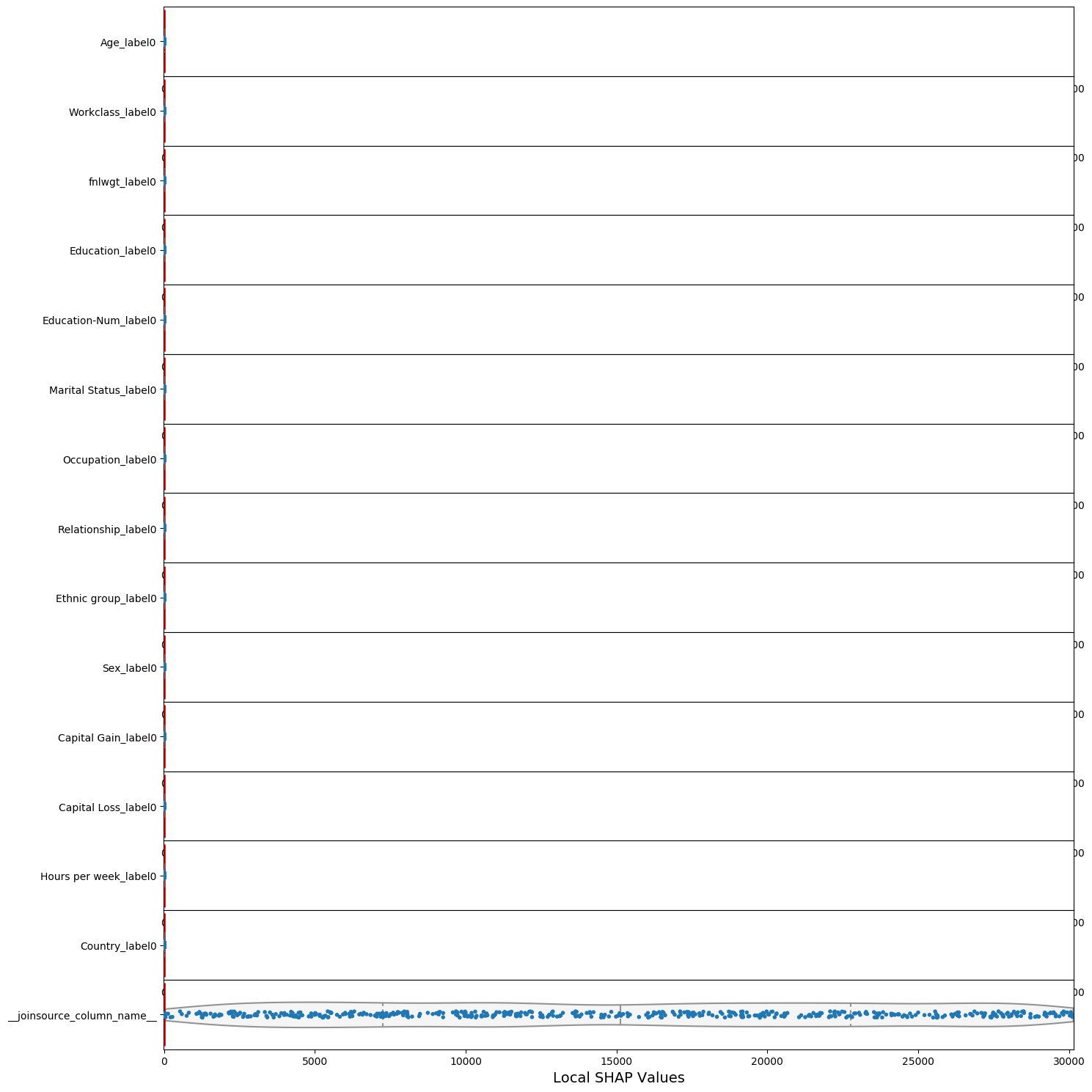
Visualize local SHAP values
[26]:
max_features_to_display = 15
feature_names = local_shap_values.columns

fig = plt.figure(figsize=(max_features_to_display, max_features_to_display))
low = local_shap_values.min().min()
high = local_shap_values.max().max()

i = 1
for feature_name in feature_names:
    plt.subplot(max_features_to_display, 1, i)
    shap_value = local_shap_values[f"{feature_name}"].to_frame()
    feature = pd.Series([feature_name] * shap_value.shape[0]).to_frame()
    df = pd.concat([shap_value, feature], axis=1, join="inner", ignore_index=True)
    df.columns = ["shap_value", "feature"]
    num_rows_to_display = min(df.shape[0], 500)
    df = df.sample(num_rows_to_display)
    ax = sns.violinplot(
        y="feature",
        x="shap_value",
        data=df,
        size=6,
        color="#f5f5f5",
        inner="quartile",
        bw=0.2,
        cut=0,
        orient="h",
    )
    ax.set_xlim(low, high)
    sns.stripplot(
        y="feature",
        x="shap_value",
        data=df,
        size=4,
        orient="h",
    )
    ax.vlines(0, -1, 1, color="#ff0000", linewidth=2)
    ax.set_ylabel("")
    ax.legend([], [], frameon=False)
    i += 1


plt.xlabel("Local SHAP Values", fontsize=14)
plt.tight_layout()
plt.subplots_adjust(hspace=0, wspace=0.1)

plt.show()
Note: You can run both bias and explainability jobs at the same time with run_bias_and_explainability(), refer API Documentation for more details.
Clean Up
Finally, don’t forget to clean up the resources we set up and used for this demo!
[28]:
sagemaker_session.delete_model(model_name)
INFO:sagemaker:Deleting model with name: DEMO-clarify-model-07-02-2023-03-52-02
Notebook CI Test Results
This notebook was tested in multiple regions. The test results are as follows, except for us-west-2 which is shown at the top of the notebook.