Timeseries Data Flow example
This example provide quick walkthrough of how to aggregate and prepare data for Machine Learning using Amazon SageMaker Data Wrangler for Timeseries dataset.
New York city(NYC) yellow cab time-series example
Our end goal for this lab is to prepare a time-series dataset and get it to a ready state for ML modeling. We will start with the New York city (NYC) yellow cab time-series dataset and work towards exploring, preparing and transforming the dataset to help us design a ML model that will predict the number of NYC yellow taxi pickups for any hour of the day and location. As part of the exercise, we will learn how to derive various insights about the trip like average tip value, average distance for the trip, etc.
Data used in this demo: - Original data source for all open data from 2008 to Current can be accessed here: https://www1.nyc.gov/site/tlc/about/tlc-trip-record-data.page - AWS-hosted location: https://registry.opendata.aws/nyc-tlc-trip-records-pds/
The taxi trip records include fields capturing pick-up and drop-off dates/times, pick-up and drop-off locations, trip distances, itemized fares, rate types, payment types, and driver-reported passenger counts. The raw data is split 1 month per file, per Yellow, Green, or ForHire from 2008 through 2020, with each file around 600 MB. The entire raw dataset is huge. For our lab, we will use 13 of these files of around a year’s worth of trip data and focus only on the iconic yellow cab trips. We picked trip data from Feb 2019 to Feb 2020 to avoid COVID effects. The data dictionary below describes the Yellow taxi trip data with raw feature column names and their respective descriptions. The picked dataset covers 13 months and encapsulates approximately 90 million trips.
Instructions to download the dateset
You can use SageMaker Data Wrangler to import data from the following data sources: Amazon Simple Storage Service (Amazon S3), Amazon Athena, Amazon Redshift, and Snowflake. The dataset that you import can include up to 1000 columns. For this lab, we will be using Amazon S3 as the preferred data source. Before we import the dataset into SageMaker Data Wrangler, let’s ensure we copy the dataset first from the publicly hosted location to our local S3 bucket in our own account.
To copy the dataset, copy and execute the Python code below within SageMaker Studio. It is recommended to execute this code in a notebook setting. We also recommend to have your S3 bucket in the same region as SageMaker Data Wrangler.
To create a SageMaker Studio notebook, from the launcher page, click on the Notebook Python 3 options under Notebooks and compute resources as show in the figure below.
Copy and paste the shared code snippet below into the launched notebook’s cell (shown below) and execute it by clicking on the play icon on the top bar.
import boto3
import json


# Setup
REGION = 'us-east-1'
account_id = boto3.client('sts').get_caller_identity().get('Account')
bucket_name = f'{account_id}-{REGION}-dw-ts-lab'


# Create S3 bucket to download dataset in your account
s3 = boto3.resource('s3')

if REGION == 'us-east-1':
    s3.create_bucket(Bucket=bucket_name)
else:
    s3.create_bucket(Bucket=bucket_name,CreateBucketConfiguration={'LocationConstraint': REGION})
    # Copy dataset from public hosted location to your S3 bucket
trips = [
    {'Bucket': 'nyc-tlc', 'Key': 'trip data/yellow_tripdata_2019-02.parquet'},
    {'Bucket': 'nyc-tlc', 'Key': 'trip data/yellow_tripdata_2019-03.parquet'},
    {'Bucket': 'nyc-tlc', 'Key': 'trip data/yellow_tripdata_2019-04.parquet'},
    {'Bucket': 'nyc-tlc', 'Key': 'trip data/yellow_tripdata_2019-05.parquet'},
    {'Bucket': 'nyc-tlc', 'Key': 'trip data/yellow_tripdata_2019-06.parquet'},
    {'Bucket': 'nyc-tlc', 'Key': 'trip data/yellow_tripdata_2019-07.parquet'},
    {'Bucket': 'nyc-tlc', 'Key': 'trip data/yellow_tripdata_2019-08.parquet'},
    {'Bucket': 'nyc-tlc', 'Key': 'trip data/yellow_tripdata_2019-09.parquet'},
    {'Bucket': 'nyc-tlc', 'Key': 'trip data/yellow_tripdata_2019-10.parquet'},
    {'Bucket': 'nyc-tlc', 'Key': 'trip data/yellow_tripdata_2019-11.parquet'},
    {'Bucket': 'nyc-tlc', 'Key': 'trip data/yellow_tripdata_2019-12.parquet'},
    {'Bucket': 'nyc-tlc', 'Key': 'trip data/yellow_tripdata_2020-01.parquet'},
    {'Bucket': 'nyc-tlc', 'Key': 'trip data/yellow_tripdata_2020-02.parquet'}
]
for trip in trips:
    s3.meta.client.copy(trip, bucket_name, trip['Key'])
Now we have raw data in our S3 bucket and ready to explore it and build a training dataset
Dataset Import
Our first step is to launch a new SageMaker Data Wrangler session and there are multiple ways how to do that. For example, use the following:
Click File -> New -> Data Wrangler Flow
Amazon SageMaker will start to provision a resources for you and you a could find a new Data Wrangler Flow file in a File Browser section
Lets rename our new workflow: Right click on file -> Rename Data Wrangler Flow
Put a new name, for example: TS-Workshop-DataPreparation.flow
In few minutes Data Wrangler will finish to provision resources and you could see “Import Data” screen. SageMaker Data Wrangler supports many data sources: Amazon S3, Amazon Athena, Amazon Redshift, Snowflake, Databricks. Our data already in S3, let’s import it by clicking “Amazon S3” button.
You will see all your S3 buckets so please search for your bucket (if you used provided code the bucket will have a suffix dw-ts-lab)
All the files required for this lab are in “trip data” folder, so let’s select it. SageMaker Data Wrangler will import all files from a folder and sample up to 100 MB of data for an interactive preview. On a right side menu you could customize import job settings like Name, File type, Delimiter, etc. More information about import process could be found here.
To finish setting up import step select “parquet” in “File type” drop down menu and press the orange button “Import”
It will take a few minutes to import data and validate it. SageMaker Data Wrangler will automatically recognize data types. You should see “Validation complete 0 errors message”
Change data types
First we will check the data types were correctly recognized. This might be necessary as Data Wrangler selects data types based on a sampled data which is limited to 50000 rows. Sampled data might potentially miss some variations.
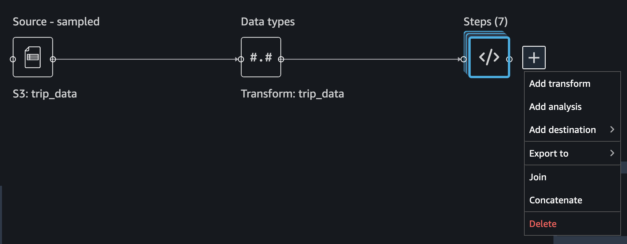
To add a data transformation step use the plus sign next to Data types and choose Edit data types as shown below.
In our case several columns were incorrectly recognized: -
passenger_count (must be long instead of float) -
RatecodeID (must be long instead of float) - airport_fee
(must be float instead of long)
I know correct data types from dataset description. In real life you could also easily find such information. Let’s correct data types by selecting a correct type from a drop down menu.
Click Preview and then Apply button.
Click Back to data flow.
Dataset preparation
Drop columns
Before we analyze data and do feature engineering we have to clean dataset and below steps show how to remove unwanted data.
To re-iterate our business goal: Predict the number of NY City yellow taxi pickups in the next 24 hour for each pickup per hour zones and provide some insights for drivers like average tips, average distance, etc.
As we are interested in per hour forecast we have to aggregate some features and remove features which are impossible to aggregate. For this purpose we don’t need the following columns:
VendorID(A code indicating the TPEP provider that provided the record)RatecodeID(The final rate code in effect at the end of the trip)Store_and_fwd_flag(This flag indicates whether the trip record was held in vehicle memory before sending to the vendor, aka “store and forward,”because the vehicle did not have a connection to the server)DOLocationID(TLC Taxi Zone in which the taximeter was disengaged)Payment_type(A numeric code signifying how the passenger paid for the trip)Fare_amount(The time-and-distance fare calculated by the meter) - we will use total amount featureExtra(Miscellaneous extras and surcharges)MTA_tax(0.50 MTA tax that is automatically triggered based on the metered rate in use)Tolls_amount(Total amount of all tolls paid in trip)Improvement_surcharge(improvement surcharge assessed trips at the flag drop. The improvement surcharge began being levied in 2015)Passenger_count(This is a driver-entered value)congestion_surcharge(Total amount collected in trip for NYS congestion surcharge)Airport_fee(Only at LaGuardia and John F. Kennedy Airports)
To remove those columns: 1. Click the plus sign next to “Data types” element and choose Add transform.

Click “+ Add step” orange button in the TRANSFORMS menu.
- Choose Manage columns.
For Transform, choose Drop column and for Column to drop, choose all mentioned above.
Choose Preview
Choose Add to save the step.
Once transformation is applied on a sampled data you should see all current steps and a preview of a resulted dataset like show here.
Click Back to data flow.
Handle missing and invalid data in timestamps
Missing data is a common problem in real life, it could be a result of data corruption, data loss or issues in data ingestion. The best practice is to verify the presence of any missing or invalid values and handle them appropriately.
There are many different strategies how missing or invalid data could be handled, for example dropping rows with missing values or filling the missing values with static or calculated values. Depending on dataset size you could choose what to do: fix values or just drop them. The Time Series - Handle missing transform allows you to choose from multiple strategies.
All future aggregations will be based on time stamps, so we have to make
sure that we don’t have any rows with missing time stamps (
tpep_pickup_datetime and tpep_dropoff_datetime features).
SageMaker Data Wrangler has several time series specific
transformations, including Validate timestamps which checks for
scenarios: 1. Checking timestamp column for any missing values. 2.
Validate the timestamp columns for the desired timestamp format.
To validate timestamps in tpep_dropoff_datetime and
tpep_pickup_datetime columns: 1. Click the plus sign next to “Drop
columns” element and choose Add transform.

Click “+ Add step” orange button in the TRANSFORMS menu.
Choose Time Series.
For Transform choose Validate Timestamps, For TimeStamp columns choose
tpep_pickup_datetime, for Policy select drop.Choose Preview
Choose Add to save the step.
Repeat same steps again for
tpep_dropoff_datetimecolumn
When you apply a transformation a sampled data you should see all current steps and a preview of a resulted dataset.
Click Back to data flow.
Feature engineering based on a timestamp with a custom transformation.
At this stage we have pickup and drop-off timestamps, but we are more
interested in pickup timestamp and ride duration. We have to create a
new feature ride duration as a difference between pick up and drop
off time in minutes. There is no built-in date difference transformation
in a Data Wrangler, but we could create it with a custom transformation.
The Custom Transforms allows you to use Pyspark, Pandas, or Pyspark
(SQL) to define your own transformations. For all three options, you use
the variable df to access a dataframe to which you want to apply the
transform. You do not need to include a return statement.
To create a custom transformation you have to: 1. Click the plus sign next to a collection of transformation elements and choose Add transform.
Click “+ Add step” orange button in the TRANSFORMS menu.
Choose Custom transform.
Name the transformation as “Duration_Transformation” - (naming is optional but good to have a structure)
In drop down menu select Python (PySpark) and use code below. This code will import functions, calculate difference between two timestamps by converting them to unix format (real number) and round result and drop tpep_dropoff_datetime column
from pyspark.sql.functions import col, round
df = df.withColumn('duration', round((col("tpep_dropoff_datetime").cast("long")-col("tpep_pickup_datetime").cast("long"))/60,2))
df = df.drop("tpep_dropoff_datetime")
Choose Preview
Choose Add to save the step.
When transformation is applied on a sampled data you should see all current steps and a preview of a resulted dataset with a new column duration and without column tpep_dropoff_datetime
Click Back to data flow.
Handling missing data in numeric attributes
We already discussed what are missing values and why it is important to
handle them. So far, we have been working with timestamps only. Now, we
are going to handle missing values in the rest of attributes. We can
exclude duration feature from this operation as it was calculated
from timestamps in the previous step. As we discussed before, there are
several ways to handle missing data: fill a static number or calculate a
value (for example: median or mean for last 7 days). It might make sense
to calculate a value if your time-series represents a continuous process
like sensor reading or product sale quantity. In our case, all trips are
independent from each other and we cannot calculate values based on
previous trips as it might bring data bias and increase error. We can
replace missing values with zeros or sometimes it might make sense to
drop the entire row with missing values.
Amazon Data Wrangler has two types of transformations to handle missing data: i) generic and ii) specifically designed for time series data. Here, we demonstrate how to use both of them and describe when to use each of these transformations.
Handle missing data with the generic “Handle missing values” transformations
This transformation can be used if you want to: 1. Replace missing values with a same static value for all time series 2. Replace missing values with a calculated value and you have only one time series (for example: one sensor or one product in a shop)
To create this transformation you have to: 1. Click the plus sign next to a collection of transformation elements and choose Add transform.

Click “+ Add step” orange button in the TRANSFORMS menu.
Choose Handle Missing
For “Transform” choose Fill missing
For “inputs columns” choose
PULocationID,tip_amount, andtotal_amountFor “Fill value” put 0
Choose Preview
Choose Add to save the step.
When transformation is applied on a sampled data you should see all current steps and a preview of a resulted dataset.
Handle missing data with special Time Series transformation
In real life datasets, we have many time-series in the same dataset and to separate them, we use some form of IDs. For example, sensor ID or item SKU. If we want to replace missing values with calculated values, for example mean for last 10 sensor observations, we must calculate it based on data for each time series independently. Instead of writing code, you could use the special Time Series transformation in Data Wrangler and get this easily done!.
To create this transformation you have to: 1. Click “+ Add step” orange button in the TRANSFORMS menu.

Choose Time Series
For “Transform” choose Handle missing
For “Time series input type” choose Along column
For “Impute missing values for this column” choose
trip_distanceFor “Timestamp column” choose tpep_pickup_datetime
For “ID column” choose PULocationID
For “Method for imputing values” choose Constant value
For “Custom value” put 0.0
Choose Preview
Choose Add to save the step.
When this transformation is applied on the dataset, you can see all current steps until this point in time and get a preview of the resulting dataset.
Filter rows with invalid data
Based on our understanding of the dataset until this point, we could also apply several filters to remove invalid or corrupt data from a business point of view. This will improve data quality even further and ensure we feed only correct data to our model training process.
We can filter data based on following rules: 1. tpep_pickup_datetime
- have to be in range from 1 Jan 2019 (included) till 1 March 2020
(excluded) 2. trip_distance - have to be greater than or equal to 0
(only positive numbers) 3. tip_amount - have to be greater than or
equal to 0 (only positive numbers) 4. total_amount - have to be
greater than or equal to 0 (only positive numbers) 5. duration -
have to be greater than or equal to 1 (we are not interested in super
short trips). 6. PULocationID - have to be in the range (1 to 263).
These are the assigned zones. For the sake of brevity, let’s use only
the 1st ten location IDs for this workshop (see image below).
There is no built-in filter transformation in Data Wrangler to handle these various constraints. Hence, we will create a custom transformation.
To create a custom transformation, follow the steps below: 1. Click the plus sign next to a collection of transformation elements and choose Add transform.

Click “+ Add step” orange button in the TRANSFORMS menu.
Choose Custom Transform.
In drop down menu select Python (PySpark) and use code below. This code will filter rows based on the specified conditions.
df = df.filter(df.trip_distance >= 0)
df = df.filter(df.tip_amount >= 0)
df = df.filter(df.total_amount >= 0)
df = df.filter(df.duration >= 1)
df = df.filter((1 <= df.PULocationID) & (df.PULocationID <= 263))
df = df.filter((df.tpep_pickup_datetime >= "2019-01-01 00:00:00") & (df.tpep_pickup_datetime < "2020-03-01 00:00:00"))
Choose Preview
Choose Add to save the step.
When this transformation is applied on the dataset, you can see all current steps until this point in time and get a preview of the resulting dataset.
Quick analysis of dataset
Amazon SageMaker Data Wrangler includes built-in analysis that help you generate visualizations and data insights in a few clicks. You can either leverage the built-in analyses types we offer out of the box with the product or create your own custom analysis using your own code if needed. SageMaker Data Wrangler also provides automated insights by automatically performing exploratory and descriptive analyses behind the scenes on your data. It identifies hidden anomalies and red flags within your dataset and proposes prescriptive actions in the form of what transforms can be applied on what columns of your data to fix these issues.
For this lab, let’s use the Table Summary built-in analysis type to
quickly summarize our existing dataset in its current form. For the
numeric columns, including long and float data, table summary reports
the number of entries (count), minimum (min), maximum (max),
mean, and standard deviation (stddev) for each column. For columns
with non-numerical data, including columns with String, Boolean, or
DateTime data, table summary reports the number of entries (count),
least frequent value (min), and most frequent value (max).
To create this analysis, follow the steps below: 1. Click the plus sign next to a collection of transformation elements and choose “Add analyses”.
In a “analyses type” drop down menu select “Table Summary” and provide a name for “Analysis name”, for example: “Cleaned dataset summary”
Choose Preview
Choose Add to save the analyses.
You could find your first analyses on a “Analysis” tab. All future visualizations will could be also found here.
Click on analyses icon to open it.
Let’s take a look at our results. The most interesting part is the summary for duration column: maximum value is 1439 and this is in minutes! 1439 minutes = almost 24 hours and this is definitely an issue which will reduce the quality of our model if this dataset is used in its current form. This looks more like an issue due to the prevalence of outliers in our dataset. Next, let’s see how to issue this issue using a built-in transform Data Wrangler offers.
Handling outliers in numeric attributes
In statistics, an outlier is a data point that differs significantly
from other observations in the same dataset. An outlier may be due to
variability in the measurement or it may indicate experimental error.
The latter are sometimes excluded from the dataset. For example, in our
dataset we have the tip_amount feature and usually it is less than
10 dollars, but due to an error in a data collection, some values can
show thousands of dollar as a tip. Such data errors will skew statistics
and aggregated values which will lead to a lower model accuracy.
An outlier can cause serious problems in statistical analysis. Machine learning models are sensitive to the distribution and range of feature values. Outliers, or rare values, can negatively impact model accuracy and lead to longer training times. When you define a Handle outliers transform step, the statistics used to detect outliers are generated on the data available in Data Wrangler when defining this step. These same statistics are used when running a Data Wrangler job.
SageMaker Data Wrangler supports several outliers detection and handle methods. We are going to use Standard Deviation Numeric Outliers and we remove all outliers as our dataset is big enough. This transform detects and fixes outliers in numeric features using the mean and standard deviation. You specify the number of standard deviations a value must vary from the mean to be considered an outlier. For example, if you specify 3 for standard deviations, a value falling more than 3 standard deviations from the mean is considered an outlier.
To create this transformation, follow the steps below: 1. Click the plus sign next to a collection of transformation elements and choose “Add transform”.

Click “+ Add step” orange button in the TRANSFORMS menu.
Choose Handle Outliers.
For “Transform” choose “Standard deviation numeric outliers”
For “Inputs columns” choose
tip_amount,total_amount,duration, andtrip_distanceFor “Fix method” choose “Remove”
For “Standard deviations” put 4
Choose Preview
Choose Add to save the step.
When transformation is applied on a sampled data you should see all current steps and a preview of resulted dataset.
Optional: If you want, you could repeat the steps from our previous
analysis (“Quick analysis of a current dataset”) to create a new table
summary and check for the new maximum for the duration column. You
can see, the new max value for duration is 243 minutes = just over an
hour. This is more realistic for long trips than what we previously had.
Grouping/Aggregating data
At this moment we have cleaned dataset by removing outliers, invalid values, and added new features. There are few more steps before we start training our forecasting model.
As we are interested in a hourly forecast we have to count number of trips per hour per station and also aggregate (with mean) all metrics such as distance, duration, tip, total amount.
Truncating timestamp
We don’t need minutes and seconds in out timestamp, so we remove them. There is no built-in filter transformation in SageMaker Data Wrangler, so we create a custom transformation.
To create a custom transformation, follow the steps below:: 1. Click the plus sign next to a collection of transformation elements and choose “Add transform”.

Click “+ Add step” orange button in the TRANSFORMS menu.
Choose Custom Transform.
In drop down menu select Python (PySpark) and use code below. This code will create a new column with a truncated timestamp and then drop original pickup column.
from pyspark.sql.functions import col, date_trunc
df = df.withColumn('pickup_time', date_trunc("hour",col("tpep_pickup_datetime")))
df = df.drop("tpep_pickup_datetime")
Choose Preview
Choose Add to save the step
When you apply the transformation on sampled data, you can see all the
current steps until this point in time and get a preview of the
resulting dataset with a new column pickup_time and without the old
column tpep_pickup_datetime
Count number of trips per hour per station
Currently, we have only piece of information about each trip, but we don’t know how many trips were made from each station per hour. The simplest way to do that is count number of records per stationID per hourly timestamp. While Amazon Data Wrangler provides GroupBy transformation. The built-in transformation doesn’t support grouping by multiple columns, so we use a custom transformation.
To create a custom transformation you have to: 1. Click the plus sign next to a collection of transformation elements and choose “Add transform”.
Click “+ Add step” orange button in the TRANSFORMS menu.
Choose Custom Transform.
In drop down menu select Python (PySpark) and use code below. This code will create a new column with a number of trips from each location for each timestamp.
from pyspark.sql import functions as f
from pyspark.sql import Window
df = df.withColumn('count', f.count('duration').over(Window.partitionBy([f.col("pickup_time"), f.col("PULocationID")])))
Choose Preview
Choose Add to save the step.
When transformation is applied on a sampled data you should see all current steps and a preview of a resulted dataset with a new column count.
Resample time series
Now, we are ready to make a final aggregation! We want to aggregate all
rows by a combination of PULocationID and pickup_time columns,
while features should be replaced by mean value for each combination.
We use special built-in Time Series transformation Resample. The Resample transformation changes the frequency of the time series observations to a specified granularity. It also comes with both upsampling and downsampling options. Applying upsampling increases the frequency of the observations, for example from daily to hourly, whereas downsampling decreases the frequency of the observations, for example from hourly to daily.
To create this transformation, follow the steps below: 1. Click the plus sign next to a collection of transformation elements and choose Add transform.

Click “+ Add step” orange button in the TRANSFORMS menu.
Choose Time Series.
For “Transform” choose “Resample”
For “Timestamp” choose
pickup_timeFor “ID column” choose
PULocationIDFor “Frequency unit” choose “Hourly”
For “Frequency quantity” put 1
For “Method to aggregate numeric values” choose “mean”
Use default values for the rest of parameters
Choose Preview
Choose Add to save the step.
When transformation is applied on a sampled data you should see all current steps and a preview of a resulted dataset.
Resample time series
Now we are ready to make a final aggregation! We aggregate all rows by
combination of PULocationID and pickup_time timestamp while
features should be replaced by mean value for each combination.
We use special built-in Time Series transformation Resample. The Resample transformation changes the frequency of the time series observations to a specified granularity. It also comes with both upsampling and downsampling options. Applying upsampling increases the frequency of the observations, for example from daily to hourly, whereas downsampling decreases the frequency of the observations, for example from hourly to daily.
To create this transformation you have to: 1. Click the plus sign next to a collection of transformation elements and choose Add transform.
Click “+ Add step” orange button in the TRANSFORMS menu.
Choose Time Series.
For “Transform” choose “Resample”
For “Timestamp” choose pickup_time
For “ID column” choose “PULocationID”
For “Frequency unit” choose “Hourly”
For “Frequency quantity” put 1
For “Method to aggregate numeric values” choose “mean”
Use default values for the rest of parameters
Choose Preview
Choose Add to save the step.
When this transformation is applied on the dataset, you can see all current steps until this point in time and get a preview of the resulting dataset.
here.
Featurize Date Time
“Featurize datetime” time series transformation will add the month, day of the month, day of the year, week of the year, hour and quarter features to our dataset. Because we’re providing the date/time components as separate features, we enable ML algorithms to detect signals and patterns for improving prediction accuracy.
To create this transformation you have to: 1. Click the plus sign next to a collection of transformation elements and choose Add transform
Click “+ Add step” orange button in the TRANSFORMS menu
Choose Time Series
For “Transform” choose “Featurize date/time”
For “Input Column” choose
pickup_timeFor “Output Column” enter “date”
For “Output mode” choose “Ordinal”
For “Output format” choose “Columns”
For date/time features to extract, select Year, Month, Day, Hour, Week of year, Day of year, and Quarter.
Choose Preview
Choose Add to save the step.
When this transformation is applied on the dataset, you can see all current steps until this point in time and get a preview of the resulting dataset.
Click “Back to data flow” to head back to the block diagram editor window.
Lag feature
Next let’s create lag features for the target column count. Lag features in time-series analysis are values at prior timestamps that are considered helpful in inferring future values. They also help identify autocorrelation, also known as serial correlation, patterns in the residual series by quantifying the relationship of the observation with observations at previous time steps. Autocorrelation is similar to regular correlation but between the values in a series and its past values. It forms the basis for the autoregressive forecasting models in the ARIMA series.
With SageMaker Data Wrangler’s Lag feature transform, you can easily create lag features n periods apart. Additionally, we often want to create multiple lag features at different lags and let the model decide the most meaningful features. For such a scenario, the Lag features transform helps create multiple lag columns over a specified window size.
To create this transformation, follow the steps below: 1. Click the plus sign next to a collection of transformation elements and choose Add transform.
Click “+ Add step” orange button in the TRANSFORMS menu.
Choose Time Series
For “Transform” choose “Lag features”
For “Generate lag features for this column” choose “count”
For “ID column” enter “PULocationID”
For “Timestamp Column” choose “pickup_time”
For Lag, enter 8. You could try to use different values, maybe 24 hours in our case makes more sense.
Because we’re interested in observing up to the previous 8 lag values, let’s select Include the entire lag window.
To create a new column for each lag value, select Flatten the output
Choose Preview
Choose Add to save the step.
When transformation is applied on a sampled data you should see all current steps and a preview of a resulted dataset.
Rolling window features
We can also calculate meaningful statistical summaries across a range of values and include them as input features. Let’s extract common statistical time series features.
Data Wrangler implements automatic time series feature extraction
capabilities using the open source tsfresh package. With the time
series feature extraction transforms, you can automate the feature
extraction process. This eliminates the time and effort otherwise spent
manually implementing signal processing libraries. We will extract
features using the Rolling window features transform. This method
computes statistical properties across a set of observations defined by
the window size.
To create this transformation you have to: 1. Click the plus sign next to a collection of transformation elements and choose Add transform
Click “+ Add step” orange button in the TRANSFORMS menu.
Choose Time Series
For “Transform” choose “Rolling window features”
For “Generate rolling window features for this column” choose “count”
For “Timestamp Column” choose “pickup_time”
For “ID column” enter
PULocationIDFor “Window size”, enter 8. You could try to use different values, maybe 24 hours in our case makes more sense.
Select Flatten to create a new column for each computed feature.
Choose “Strategy” as “Minimal subset”. This strategy extracts eight features that are useful in downstream analyses. Other strategies include Efficient Subset, Custom subset, and All features.
Choose Preview
Choose Add to save the step.
When this transformation is applied on the dataset, you can see all current steps until this point in time and get a preview of the resulting dataset.
Click “Back to data flow” to head back to the block diagram editor window.
Export Data
At this stage, we have a new dataset that is cleaned and transformed with newly engineered features. This dataset can be used for forecasting either using open source libraries/frameworks or AWS services like Amazon SageMaker Autopilot, Amazon SageMaker Canvas or Amazon Forecast.
Given, we had only used a sample of the dataset for creating our data preparation and transformation recipe so far, what need to do next is to apply the same recipe (data flow) on our entire dataset and scale the whole process in a distributed fashion. Amazon Data Wrangler let’s you do this in multiple ways. You can export your data flow: 1/ as a processing job, 2/ as a SageMaker pipeline step, or 3/ as a Python script. You can also kick-off these distributed jobs via the UI without writing any code using Data Wrangler’s destination node option. The export options are also facilitated via SageMaker Studio notebooks (Jupyter). Additionally, the transformed features can also be ingested directly to SageMaker Feature Store.
For this lab, we will see how to use the destination nodes option to export the transformed features to S3 via a distributed PySpark job powered by SageMaker Processing.
Exporting to S3 using Destination Nodes
This option creates a SageMaker processing job which uses the data flow (recipe) we have created previously to kick-off a distributed processing job on the “entire” dataset saving the results to a specified S3 bucket.
Additionally, you can also drop columns if needed right before the
export step. For the sake of brevity and to simplify the prediction
problem statement, let’s drop all columns except three columns
pickup_time, count, PULocationID. Here count is the target
variable we will try to predict. pickup_time and PULocationID
will be our feature columns used for modeling. To create the model, we
will be using SageMaker Autopilot. This will be covered in the next 2
sections.
Follow the next steps to setup export to S3. 1. Click the plus sign next to a collection of transformation elements and choose “Add destination” -> “Amazon S3”

Provide parameters for S3 destination:
Dataset name - name for new dataset, for example used “NYC_export”
File type - CSV
Delimiter - Comma
Compression - none
Amazon S3 location - You can use the same bucket name which we created at the beginning
Click “Add destination” orange button
Now your dataflow has a final step and you see a new “Create job” orange button. Click it.
Provide a “Job name” or keep autogenerated option and select “destination”. We have only one “S3:NYC_export”, but you might have multiple destinations from different steps in your workflow. Leave a “KMS key ARN” field empty and click “Next” orange button.
Now your have to provide configuration for a compute capacity for a job. You can keep all defaults values:
For Instance type use “ml.m5.4xlarge”
For Instance count use “2”
You can explore “Additional configuration”, but keep them without change.
Click “Run” orange button
Now your job is started and it takes about 1 hour to process 6 GB of data according to our Data Wrangler processing flow. Cost for this job will be around 2 USD as “ml.m5.4xlarge” cost 0.922 USD per hour and we are using two of them.
If you click on the job name you will be redirected to a new window with the job details. On the job details page you see all parameters from a previous steps.
Approximately in one hour you should see that job status changed to “Completed” and you could also check “Processing time (seconds)” value.
Now you could close job details page.
Check Processed output
After the SageMaker Data Wrangler processing job is completed, we can check the results saved in our destination S3 bucket.
At this stage, you have designed a data flow for data processing and feature engineering and successfully launched it. Of course it is not mandatory to always run a job by clicking on the “Run” button. You could also automate it, but this is a topic of another workshop in this series!
💡 Congratulations! You reached the end of this part. Now you know how to use Amazon SageMaker Data Wrangler for time series dataset preparation!
Import Dataflow
Here is the final Flow file available which you can directly import to expediate the process or validate the flow.
Here are the steps to import the flow
Download the flow file
In Sagemaker Studio, drag and drop the flow file or use the upload button to browse the flow and upload
Clean up
Delete artifacts in S3.
Delete data flow file in SageMaker Studio.
Stop active SageMaker Data Wrangler instance.
Delete SageMaker user profile and domain (optional).