Digital Farming with Amazon SageMaker Geospatial Capabilities - Part II
This notebook’s CI test result for us-west-2 is as follows. CI test results in other regions can be found at the end of the notebook.
In this notebook, we continue explore some of most common tasks for processing geospatial data in the Digital Farming domain, by working with Amazon SageMaker geospatial capabilities.
Environment Set-Up
We will start by making sure the “sagemaker” SDK is updated, and importing a few libraries required.
[ ]:
# Install Reinvent Wheels
!pip install sagemaker --upgrade
!pip install rasterio
[ ]:
import boto3
import sagemaker

import json
from datetime import datetime
import rasterio
from rasterio.plot import show
from matplotlib import pyplot as plt
import time
[ ]:
sagemaker_session = sagemaker.Session()
bucket = sagemaker_session.default_bucket()  ### Replace with your own bucket if needed
role = sagemaker.get_execution_role(sagemaker_session)
sess = boto3.Session()
prefix = "sm-geospatial-e2e"  ### Replace with the S3 prefix desired
print(f"S3 bucket: {bucket}")
print(f"Role: {role}")
Make sure you have the proper policy and trust relationship added to your role for “sagemaker-geospatial”, as specified in the Get Started with Amazon SageMaker Geospatial Capabiltiies documentation.
[ ]:
gsClient = boto3.client("sagemaker-geospatial")
Other common geospatial processing tasks for Digital Farming
We will save the ARN of our collection of interest. In our example we will work with satellite imagery data from the Sentinel-2-L2A collection…
[ ]:
data_collection_arn = "arn:aws:sagemaker-geospatial:us-west-2:378778860802:raster-data-collection/public/nmqj48dcu3g7ayw8"
### Replace with the ARN of the collection of your choice
First, we will define the input configuration with the polygon of coordinates for our area of interest and the time range we are interested on.
[ ]:
### Replace with the coordinates for the polygon of your area of interest...
coordinates = [
    [9.742977, 53.615875],
    [9.742977, 53.597119],
    [9.773620, 53.597119],
    [9.773620, 53.615875],
    [9.742977, 53.615875],
]
### Replace with the time-range of interest...
time_start = "2022-03-01T12:00:00Z"
time_end = "2022-03-31T12:00:00Z"
Typically, we are interested on working with images that are not covered by much clouds over our area of interest. For exploring this in our notebook, we will define some additional parameters like e.g. the ranges for cloud cover we want to consider (less than 2% in our example).
[ ]:
eoj_input_config = {
    "RasterDataCollectionQuery": {
        "AreaOfInterest": {
            "AreaOfInterestGeometry": {"PolygonGeometry": {"Coordinates": [coordinates]}}
        },
        "TimeRangeFilter": {"StartTime": time_start, "EndTime": time_end},
        "PropertyFilters": {
            "Properties": [{"Property": {"EoCloudCover": {"LowerBound": 0, "UpperBound": 2}}}]
        },
    }
}
[ ]:
eoj_input_config["RasterDataCollectionQuery"]["RasterDataCollectionArn"] = data_collection_arn


def start_earth_observation_job(eoj_name, role, eoj_input_config, eoj_config):
    # Start EOJ...
    response = gsClient.start_earth_observation_job(
        Name=eoj_name,
        ExecutionRoleArn=role,
        InputConfig=eoj_input_config,
        JobConfig=eoj_config,
    )
    eoj_arn = response["Arn"]
    print(f"{datetime.now()} - Started EOJ: {eoj_arn}")

    # Wait for EOJ to complete... check status every minute
    gs_get_eoj_resp = {"Status": "IN_PROGRESS"}
    while gs_get_eoj_resp["Status"] == "IN_PROGRESS":
        time.sleep(60)
        gs_get_eoj_resp = gsClient.get_earth_observation_job(Arn=eoj_arn)
        print(f'{datetime.now()} - Current EOJ status: {gs_get_eoj_resp["Status"]}')
    return eoj_arn
Temporal Statistics - Earth Observation Job
Following our example, we will now perform Temporal Statistics through another EOJ, this will allow consolidating the imagery of the area of interest for a given time-period.
For our example, let us consider the yearly mean, and explore the Near Infrared (NIR) band in particular.
[ ]:
eoj_config = {
    "TemporalStatisticsConfig": {
        "GroupBy": "YEARLY",
        "Statistics": ["MEAN"],
        "TargetBands": ["nir"],
    }
}

ts_eoj_arn = start_earth_observation_job(
    f'tempstatsjob-{datetime.now().strftime("%Y-%m-%d-%H-%M")}', role, eoj_input_config, eoj_config
)
Note the EOJ processing takes some minutes. We can check the status programatically by getting the EOJ with the SageMaker Geospatial client, or graphically by using the Geospatial extension for SageMaker Studio.
Stacking - Earth Observation Job
Following our example, we will now perform a band stacking through another EOJ. This allow us to combine bands together for obtaining different types of observations.
In our case, we will generate the composite image of the Red, Green, and Blue (RGB) bands for obtaining the natural or true color image of the area of interest.
[ ]:
eoj_config = {
    "StackConfig": {
        "OutputResolution": {"Predefined": "HIGHEST"},
        "TargetBands": ["red", "green", "blue"],
    }
}

s_eoj_arn = start_earth_observation_job(
    f'stackingjob-{datetime.now().strftime("%Y-%m-%d-%H-%M")}', role, eoj_input_config, eoj_config
)
Note the EOJ processing takes some minutes. We can check the status programatically by getting the EOJ with the SageMaker Geospatial client, or graphically by using the Geospatial extension for SageMaker Studio.
Semantic Segmentation for Land Cover Classification - Earth Observation Job
We will now explore the use of a built-in model in SageMaker Geospatial for detecting and classifying the different types of land found in the area of interest, through the Semantic Segmentation Land Cover model.
We can run an EOJ for performing the land cover classification on it. This would use the built-in model and perform the segmentation inference on our input data.
[ ]:
eoj_config = {"LandCoverSegmentationConfig": {}}

lc_eoj_arn = start_earth_observation_job(
    f'landcovermodeljob-{datetime.now().strftime("%Y-%m-%d-%H-%M")}',
    role,
    eoj_input_config,
    eoj_config,
)
Note the EOJ processing takes some minutes. We can check the status programatically by getting the EOJ with the SageMaker Geospatial client, or graphically by using the Geospatial extension for SageMaker Studio.
Exporting the Results
As mentioned before, the results of our EOJs are stored in the service and are available for chaining as input for another EOJ, but can also export these to Amazon S3 for visualizing the imagery directly.
We will define a function for exporting the results of our EOJs.
[ ]:
def export_earth_observation_job(eoj_arn, role, bucket, prefix, task_suffix):
    # Export EOJ results to S3...
    response = gsClient.export_earth_observation_job(
        Arn=eoj_arn,
        ExecutionRoleArn=role,
        OutputConfig={
            "S3Data": {"S3Uri": f"s3://{bucket}/{prefix}/{task_suffix}/", "KmsKeyId": ""}
        },
    )
    export_arn = response["Arn"]
    print(f"{datetime.now()} - Exporting with ARN: {export_arn}")
Let’s go through the EOJs created before for checking it’s status and exporting accordingly. Keep in mind each EOJ takes some minutes to complete, so we will add a check on the status every 30 seconds…
[ ]:
# Check status of EOJs...
EOJs = [ts_eoj_arn, s_eoj_arn, lc_eoj_arn]
eoj_suffixes = ["temp_stat", "stacking", "land_cover"]

eoj_status = [""] * len(EOJs)
while not all(i == "Exported" for i in eoj_status):
    # Wait for EOJs to complete and export... check status every 30 seconds
    for j, eoj in enumerate(EOJs):
        gs_get_eoj_resp = gsClient.get_earth_observation_job(Arn=eoj)
        if gs_get_eoj_resp["Status"] == "COMPLETED":
            # EOJ completed, exporting...
            if not "ExportStatus" in gs_get_eoj_resp:
                export_earth_observation_job(eoj, role, bucket, prefix, eoj_suffixes[j])
            elif gs_get_eoj_resp["ExportStatus"] == "IN_PROGRESS":
                eoj_status[j] = "Exporting"
            elif gs_get_eoj_resp["ExportStatus"] == "SUCCEEDED":
                eoj_status[j] = "Exported"
            else:
                raise Exception("Error exporting")
        elif gs_get_eoj_resp["Status"] == "IN_PROGRESS":
            # EOJ still in progress, keep waiting...
            eoj_status[j] = "In progress"
        else:
            raise Exception("Error with the EOJ")
        print(f"{datetime.now()} - EOJ: {eoj} Status: {eoj_status[j]}")
    if all(i == "Exported" for i in eoj_status):
        break
    time.sleep(30)
Now that we have all our EOJs exported, let’s visualize a few of the images obtained in S3.
For this we will use the open library “rasterio”.
[ ]:
s3 = boto3.resource("s3")
my_bucket = s3.Bucket(bucket)


def visualize_cogt(task, eoj_arn, band, number):
    gs_get_eoj_resp = gsClient.get_earth_observation_job(Arn=eoj_arn)
    if gs_get_eoj_resp["ExportStatus"] == "SUCCEEDED":
        i = 0
        for index, image in enumerate(
            my_bucket.objects.filter(
                Prefix=f'{prefix}/{task}/{eoj_arn.split("/",1)[1]}/output/consolidated/'
            )
        ):
            if f"{band}.tif" in image.key:
                i = i + 1
                tif = f"s3://{bucket}/{image.key}"
                with rasterio.open(tif) as src:
                    arr = src.read(out_shape=(src.height // 20, src.width // 20))
                    if band != "visual":
                        # Sentinel-2 images are stored as uint16 for optimizing storage
                        # but these need to be reslaced (by dividing each pixel value by 10000)
                        # to get the true reflectance values. This is a common “compression”
                        # technique when storing satellite images...
                        arr = arr / 10000
                        # As a result of the transformation, there might be some pixel values
                        # over 1 in the RGB, so we need to replace those by 1...
                        arr[arr > 1] = 1
                show(arr)
                print(tif)
                if i == number:
                    break
    else:
        print(
            f'Export of job with ARN:\n{eoj_arn}\nis in ExportStatus: {gs_get_eoj_resp["ExportStatus"]}'
        )
For the Temporal Statistics, we can check in example some of the images obtained for the mean in the NIR band.
[ ]:
visualize_cogt("temp_stat", ts_eoj_arn, "nir_mean", 4)
For the Stacking, let’s visualize the some of the stacked images for the natural color.
[ ]:
visualize_cogt("stacking", s_eoj_arn, "stacked", 4)
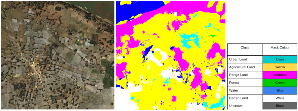
For the Land Cover classification, let’s visualize a few of the output images obtained after the built-in segmentation inference.
[ ]:
visualize_cogt("land_cover", lc_eoj_arn, "L2A", 30)
Here, take into account the legend for the segmentation the below.

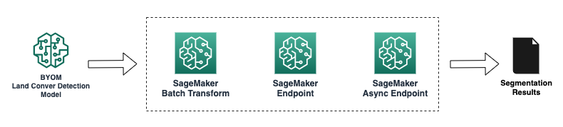
Bring-Your-Own-Model (BYOM) for Inference on Geospatial Data
In this section, we suggest a sample code to bring a pre-trained model for running inferences on the geospatial data. This is relevant when the built-in models included in the service are not sufficient for your custom use case.
For illustrating the example, the code below would allow running predictions with a model artifact you specify in the MODEL_S3_PATH parameter, by creating a SageMaker Model with the pre-trained weights, dependencies, and inference script using SageMaker in “Script-Mode”.
This allows you performing inferences using different methods, including e.g. a SageMaker Endpoint (real-time), a SageMaker Async Endpoint, or a SageMaker Batch Transform job.
NOTE: In this section you are expected to provide/upload your own model artifact, inference script, and any dependencies required for your model before uncommenting and running the cells below.
[ ]:
# from sagemaker.pytorch import PyTorchModel

# model = PyTorchModel(
#    name=model_name, ### Set a model name
#    model_data=MODEL_S3_PATH, ### Location of the custom model package (model.tar.gz) in S3
#    role=role,
#    entry_point='inference.py', ### Replace with the name of your inference entry-point script, added to the source_dir
#    source_dir='code', ### Folder with any dependencies e.g. requirements.txt file, and your inference script
#    image_uri=image_uri, ### URI for your AWS DLC or custom container URI
#    env={
#        'TS_MAX_REQUEST_SIZE': '100000000',
#        'TS_MAX_RESPONSE_SIZE': '100000000',
#        'TS_DEFAULT_RESPONSE_TIMEOUT': '1000',
#    }, ### Optional – Set environment variables for max size and timeout
# )
[ ]:
# predictor = model.deploy(
#    initial_instance_count = 1, ### Your number of instances for the endpoint
#    instance_type = 'ml.g5.xlarge', ### Your instances type for the endpoint
#    async_inference_config=sagemaker.async_inference.AsyncInferenceConfig(
#        output_path=f"s3://{bucket}/{prefix}/output",
#        max_concurrent_invocations_per_instance=2,
#    ), ### Optional – Async config if using SageMaker Async Endpoints
# )
[ ]:
# predictor.predict(data) ### Replace "data" with your images for inference
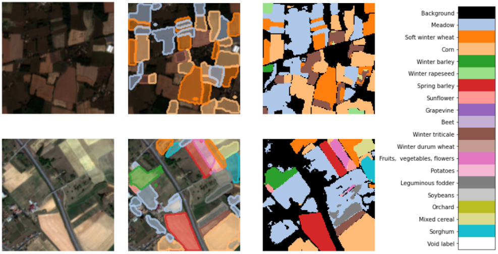
As an example, you could bring your own models for obtaining results as the below.
For a Landcover Type segmentation:
Or a Crop Type segmentation:
Clean-up
Once done, uncomment and run the following cells for deleting any resources that could incur in costs.
Delete any exported imagery in S3:
[ ]:
#!aws s3 rm s3://{bucket}/{prefix} --recursive
Delete the BYOM SageMaker Endpoint
[ ]:
# endpoint_name='<endpoint_name>' # Specify the name of your endpoint
# sagemaker_client = boto3.client('sagemaker', region_name=region)
# sagemaker_client.delete_endpoint(EndpointName=endpoint_name)
Notebook CI Test Results
This notebook was tested in multiple regions. The test results are as follows, except for us-west-2 which is shown at the top of the notebook.