Digital Farming with Amazon SageMaker Geospatial Capabilities - Part I
This notebook’s CI test result for us-west-2 is as follows. CI test results in other regions can be found at the end of the notebook.
In this notebook, we will explore some of most common tasks for processing geospatial data in the Digital Farming domain, by working with Amazon SageMaker geospatial capabilities.
Environment Set-Up
We will start by importing a few libraries required, the necessary dependencies are already pre-installed in the Geospatial kernel.
[ ]:
import boto3
import sagemaker
import sagemaker_geospatial_map

import json
from datetime import datetime
import rasterio
from rasterio.plot import show
from matplotlib import pyplot as plt
import pandas as pd
import time
We will now define a few variables for which we need to create sessions in the SageMaker and Boto3 SDKs.
We will also create the client for SageMaker geospatial capabilities by creating a Botocore session…
[ ]:
sagemaker_session = sagemaker.Session()
bucket = sagemaker_session.default_bucket()  ### Replace with your own bucket if needed
role = sagemaker.get_execution_role(sagemaker_session)
prefix = "sm-geospatial-e2e"  ### Replace with the S3 prefix desired
region = boto3.Session().region_name
print(f"S3 bucket: {bucket}")
print(f"Role: {role}")
print(f"Region: {region}")
Note, at the time of writting this notebook sagemaker-geospatial is only available in the region “us-west-2”.
Make sure you have the proper policy allowed and a trust relationship added to your role for “sagemaker-geospatial”, as specified in the Get Started with Amazon SageMaker Geospatial Capabilties documentation.
[ ]:
gsClient = boto3.client("sagemaker-geospatial", region_name=region)
Common geospatial processing tasks for Digital Farming
Now that we have the client setup, we are ready to work with SageMaker Geospatial.
We can in example check the raster collections available…
[ ]:
list_raster_data_collections_resp = gsClient.list_raster_data_collections()
list_raster_data_collections_resp["RasterDataCollectionSummaries"]
We will save the ARN of our collection of interest. In our example we will work with satellite imagery data from the Sentinel-2-L2A collection…
[ ]:
data_collection_arn = "arn:aws:sagemaker-geospatial:us-west-2:378778860802:raster-data-collection/public/nmqj48dcu3g7ayw8"
### Replace with the ARN of the collection of your choice
First, we will define the input configuration with the polygon of coordinates for our area of interest and the time range we are interested on.
[ ]:
### Replace with the coordinates for the polygon of your area of interest...
coordinates = [
    [9.742977, 53.615875],
    [9.742977, 53.597119],
    [9.773620, 53.597119],
    [9.773620, 53.615875],
    [9.742977, 53.615875],
]
### Replace with the time-range of interest...
time_start = "2022-03-01T12:00:00Z"
time_end = "2022-03-31T12:00:00Z"
We could graphically visualize this area by using the SageMaker Studio Geospatial extension, but in our case we will use an open-source library for programatically embedding a map in the notebook.
[ ]:
def get_lat_from_coordinates(coord):
    lat = []
    for i, j in enumerate(coord):
        lat.append(coord[i][1])
    return lat


def get_lon_from_coordinates(coord):
    lon = []
    for i, j in enumerate(coord):
        lon.append(coord[i][0])
    return lon
[ ]:
# Instantiate a new map and display it
Map = sagemaker_geospatial_map.create_map()
Map.set_sagemaker_geospatial_client(gsClient)

Map.render()
[ ]:
dataset = Map.add_dataset(
    {
        "data": pd.DataFrame(
            {
                "Latitude": get_lat_from_coordinates(coordinates),
                "Longitude": get_lon_from_coordinates(coordinates),
            }
        )
    },
    auto_create_layers=True
)
Typically, we are interested on working with images that are not covered by much clouds over our area of interest. For exploring this in our notebook, we will define some additional parameters like e.g. the ranges for cloud cover we want to consider (less than 2% in our example).
[ ]:
eoj_input_config = {
    "RasterDataCollectionQuery": {
        "AreaOfInterest": {
            "AreaOfInterestGeometry": {"PolygonGeometry": {"Coordinates": [coordinates]}}
        },
        "TimeRangeFilter": {"StartTime": time_start, "EndTime": time_end},
        "PropertyFilters": {
            "Properties": [{"Property": {"EoCloudCover": {"LowerBound": 0, "UpperBound": 2}}}],
        },
    }
}

data_collection_arn = "arn:aws:sagemaker-geospatial:us-west-2:378778860802:raster-data-collection/public/nmqj48dcu3g7ayw8"
We can now search for satellite images of the area of interest and visualize, as an example, the True Color Image (TCI) tiles provided by SageMaker, or any other band of interest.
Note these images are directly provided by the built-in data sources in SageMaker geospatial capabilities, like e.g. AWS Data Exchange in our case, and the query will return the locations of these image tiles in Amazon S3.
[ ]:
response = gsClient.search_raster_data_collection(**eoj_input_config, Arn=data_collection_arn)
response
[ ]:
for i, j in enumerate(response["Items"]):
    print(response["Items"][i]["Assets"]["visual"]["Href"])
    with rasterio.open(response["Items"][i]["Assets"]["visual"]["Href"]) as src:
        arr = src.read(out_shape=(src.height // 40, src.width // 40))
        show(arr)
Cloud Gap Filling - Earth Observation Job
Currently, SageMaker Geospatial supports different types of built-in processing Earth Observation Jobs (EOJs), such as:
Cloud removal
Temporal or zonal statistics
Stacking of bands
Geo-Mosaic combinations
Re-sampling
Segmentation with built-in models
etc.
Let us explore some of these techniques with an example.
In some cases we might be interested on removing the cloudy pixels of the images, this could be e.g. if we don’t have any clear observation available in the data for our area and time-range of interest. We can do this through a Cloud Removal EOJ, which would replace or fill these cloudy pixels using any of the techniques available.
For this we will setup the cloud removal parameters. This can e.g. be set to a fixed value to run your own gap filling algorithm/logic, or alternatively use a built-in interpolation type supported in the service.
[ ]:
eoj_config = {
    "CloudRemovalConfig": {"AlgorithmName": "INTERPOLATION", "InterpolationValue": "-9999"}
}
Finally, we are ready to start the EOJ with the given config. We will define a function for this purpose that will be handy for the other tasks in this notebook.
[ ]:
eoj_input_config["RasterDataCollectionQuery"]["RasterDataCollectionArn"] = data_collection_arn


def start_earth_observation_job(eoj_name, role, eoj_input_config, eoj_config):
    # Start EOJ...
    response = gsClient.start_earth_observation_job(
        Name=eoj_name,
        ExecutionRoleArn=role,
        InputConfig=eoj_input_config,
        JobConfig=eoj_config,
    )
    eoj_arn = response["Arn"]
    print(f"{datetime.now()} - Started EOJ: {eoj_arn}")

    # Wait for EOJ to complete... check status every minute
    gs_get_eoj_resp = {"Status": "IN_PROGRESS"}
    while gs_get_eoj_resp["Status"] == "IN_PROGRESS":
        time.sleep(60)
        gs_get_eoj_resp = gsClient.get_earth_observation_job(Arn=eoj_arn)
        print(f'{datetime.now()} - Current EOJ status: {gs_get_eoj_resp["Status"]}')
    return eoj_arn
[ ]:
cr_eoj_arn = start_earth_observation_job(
    f'cloudremovaljob-{datetime.now().strftime("%Y-%m-%d-%H-%M")}',
    role,
    eoj_input_config,
    eoj_config,
)
Note the EOJ processing takes some minutes. We can check the status programatically by getting the EOJ with the SageMaker Geospatial client, or graphically by using the Geospatial extension for SageMaker Studio.
Once completed, note the resulting imagery is stored in a service bucket and it can be used for chaining this to another EOJ. Also, for visualizing these images we can, if desired, copy the results of the EOJ to our own S3 location in our account by exporting it.
Check the “Exporting the Results” section of this notebook for details.
Geo Mosaic - Earth Observation Job
A common process when working with tiles of Satellite images is combining these geographically, for having a consolidated view of the whole area of interest. We can perform this through the use of a Geo Mosaic job, applicable to the output of most of the examples provided with other processing EOJs in this notebook.
For this purpose we can set the configuration as follows.
[ ]:
eoj_config = {"GeoMosaicConfig": {"AlgorithmName": "NEAR"}}

gm_eoj_arn = start_earth_observation_job(
    f'geomosaicjob-{datetime.now().strftime("%Y-%m-%d-%H-%M")}', role, eoj_input_config, eoj_config
)
Note the EOJ processing takes some minutes. We can check the status programatically by getting the EOJ with the SageMaker Geospatial client, or graphically by using the Geospatial extension for SageMaker Studio.
Band-Math - Earth Observation Job
Follwing our example, we will now perform a band-math over predefined vegetation and soil indices supported by SageMaker geospatial capabilities. Note SageMaker geospatial capabilities can perform the band-math over one or many of these indices, and supports the use of equations.
For our case let’s obtain the moisture index by using the equation below.
[ ]:
eoj_config = {
    "BandMathConfig": {
        "CustomIndices": {
            "Operations": [{"Name": "moisture", "Equation": "(nir08 - swir16) / (nir08 + swir16)"}]
        }
    }
}

bm_eoj_arn = start_earth_observation_job(
    f'bandmathjob-{datetime.now().strftime("%Y-%m-%d-%H-%M")}', role, eoj_input_config, eoj_config
)
Note the EOJ processing takes some minutes. We can check the status programatically by getting the EOJ with the SageMaker Geospatial client, or graphically by using the Geospatial extension for SageMaker Studio.
Exporting the Results
As mentioned before, the results of our EOJs are stored in the service and are available for chaining as input for another EOJ, but can also export these to Amazon S3 for visualizing the imagery directly.
We will define a function for exporting the results of our EOJs.
[ ]:
def export_earth_observation_job(eoj_arn, role, bucket, prefix, task_suffix):
    # Export EOJ results to S3...
    response = gsClient.export_earth_observation_job(
        Arn=eoj_arn,
        ExecutionRoleArn=role,
        OutputConfig={
            "S3Data": {"S3Uri": f"s3://{bucket}/{prefix}/{task_suffix}/", "KmsKeyId": ""}
        },
    )
    export_arn = response["Arn"]
    print(f"{datetime.now()} - Exporting with ARN: {export_arn}")
Let’s go through the EOJs created before for checking it’s status and exporting accordingly. Keep in mind each EOJ takes some minutes to complete, so we will add a check on the status every 30 seconds…
[ ]:
# Check status of EOJs...
EOJs = [cr_eoj_arn, gm_eoj_arn, bm_eoj_arn]
eoj_suffixes = ["cloud_removal", "geo_mosaic", "band_math"]

eoj_status = [""] * len(EOJs)
while not all(i == "Exported" for i in eoj_status):
    # Wait for EOJs to complete and export... check status every 30 seconds
    for j, eoj in enumerate(EOJs):
        gs_get_eoj_resp = gsClient.get_earth_observation_job(Arn=eoj)
        if gs_get_eoj_resp["Status"] == "COMPLETED":
            # EOJ completed, exporting...
            if not "ExportStatus" in gs_get_eoj_resp:
                export_earth_observation_job(eoj, role, bucket, prefix, eoj_suffixes[j])
            elif gs_get_eoj_resp["ExportStatus"] == "IN_PROGRESS":
                eoj_status[j] = "Exporting"
            elif gs_get_eoj_resp["ExportStatus"] == "SUCCEEDED":
                eoj_status[j] = "Exported"
            else:
                raise Exception("Error exporting")
        elif gs_get_eoj_resp["Status"] == "IN_PROGRESS":
            # EOJ still in progress, keep waiting...
            eoj_status[j] = "In progress"
        else:
            raise Exception("Error with the EOJ")
        print(f"{datetime.now()} - EOJ: {eoj} Status: {eoj_status[j]}")
    if all(i == "Exported" for i in eoj_status):
        break
    time.sleep(30)
Now that we have all our EOJs exported, let’s visualize a few of the images obtained in S3.
For this we will use the open library “rasterio”.
[ ]:
s3 = boto3.resource("s3")
my_bucket = s3.Bucket(bucket)


def visualize_cogt(task, eoj_arn, band, number):
    gs_get_eoj_resp = gsClient.get_earth_observation_job(Arn=eoj_arn)
    if gs_get_eoj_resp["ExportStatus"] == "SUCCEEDED":
        i = 0
        for index, image in enumerate(
            my_bucket.objects.filter(
                Prefix=f'{prefix}/{task}/{eoj_arn.split("/",1)[1]}/output/consolidated/'
            )
        ):
            if f"{band}.tif" in image.key:
                i = i + 1
                tif = f"s3://{bucket}/{image.key}"
                with rasterio.open(tif) as src:
                    arr = src.read(out_shape=(src.height // 20, src.width // 20))
                    if band != "visual":
                        # Sentinel-2 images are stored as uint16 for optimizing storage
                        # but these need to be reslaced (by dividing each pixel value by 10000)
                        # to get the true reflectance values. This is a common “compression”
                        # technique when storing satellite images...
                        arr = arr / 10000
                        # As a result of the transformation, there might be some pixel values
                        # over 1 in the RGB, so we need to replace those by 1...
                        arr[arr > 1] = 1
                show(arr)
                print(tif)
                if i == number:
                    break
    else:
        print(
            f'Export of job with ARN:\n{eoj_arn}\nis in ExportStatus: {gs_get_eoj_resp["ExportStatus"]}'
        )
For our Cloud Removal, we can check in example some of the images for the “blue” band
[ ]:
visualize_cogt("cloud_removal", cr_eoj_arn, "blue", 4)
For the Geo Mosaic, let’s visualize the consolidated image shown as “visual”.
[ ]:
visualize_cogt("geo_mosaic", gm_eoj_arn, "visual", 1)
For the Band Math, let’s visualize a few of the output images for the Moisture Index.
[ ]:
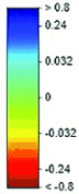
visualize_cogt("band_math", bm_eoj_arn, "moisture", 8)
Here, take into account the legend for the resulting moisture index would be similar to the below.
You can continue with the folling notebook in this series for exploring other common geospatial processing tasks.
Notebook CI Test Results
This notebook was tested in multiple regions. The test results are as follows, except for us-west-2 which is shown at the top of the notebook.