[ ]:
# Install dependencies
!pip install -q smdebug==1.0.3
!pip install -q seaborn
!pip install -q plotly
!pip install -q opencv-python
!pip install -q shap
!pip install -q bokeh
!pip install -q imageio
!pip install -Uq sagemaker
Profile machine learning training with Amazon SageMaker Debugger
This notebook’s CI test result for us-west-2 is as follows. CI test results in other regions can be found at the end of the notebook.
Gain high precision insights of horovod based distributed machine learning training jobs
Table of Contents
Section 2 - Train sentiment analysis CNN model with custom Debugger profiling configuration
Section 3 - Interactive analysis using the SMDebug visualization tools
Introduction
Training machine learning models is a time and compute intensive process requiring multiple training runs with different hyperparameters before a model yields acceptable accuracy. CPU and GPU based distributed training with frameworks such as Horovord and Parameter Servers address this issue by allowing training to be easily scalable to a cluster of resources. However, distributed training makes it harder to identify and debug resource bottleneck problems. Gaining insights into the training in progress, both at the machine learning framework level and the underlying compute resources level, is critical step towards understanding the resource usage patterns and reducing resource wastage. Analyzing bottleneck issues is necessary to maximize the utilization of compute resources and optimize model training performance to deliver state-of-the-art machine learning models with target accuracy.
Amazon SageMaker is a fully managed service that enables developers and data scientists to quickly and easily build, train, and deploy ML models at scale. Amazon SageMaker Debugger is a feature of SageMaker training that makes it easy to train machine learning (ML) models faster by capturing real-time metrics such as learning gradients and weights, providing transparency into the training process, so you can correct anomalies such as losses, overfitting, and overtraining. With the newly introduced profiling capability, SageMaker Debugger now automatically monitors system resources such as CPU, GPU, network, IO, and memory providing a complete resource utilization view of training jobs.
In this notebook, we demonstrate the Amazon SageMaker Debugger profiling capabilities using the sentiment analysis use case.
Use case - Sentiment Analysis with TensorFlow and Keras
Sentiment analysis is a very common text analytics task that involves determining whether a text sample is positive or negative about its subject. There are several different algorithms for performing this task, including statistical algorithms and deep learning algorithms. With respect to deep learning, a Convolutional Neural Net (CNN) is sometimes used for this purpose. In this notebook we’ll use a CNN built with TensorFlow to perform sentiment analysis in Amazon SageMaker on the IMDB dataset, which consists of movie reviews labeled as having positive or negative sentiment.
Step 0 - Install and check the SageMaker Python SDK version
To use the new Debugger profiling features, ensure that you have the right versions of SageMaker and SMDebug SDKs installed.
Check the library versions.
[ ]:
import sagemaker

sagemaker.__version__
Important: If the SageMaker version is less than 2.19.0 and if you are using an existing SageMaker Studio or Notebook instance, you must update the environment to use the latest SageMaker Python SDK. Follow instructions at Update Amazon SageMaker Studio and Notebook Instance Software Updates in the Amazon SageMaker developer guide.
Section 1 - Setup
In this section, you will import the necessary libraries, set up variables, and examine data to train the sentiment analysis model.
Let’s start by specifying:
The AWS region used to host your model.
The IAM role associated with this SageMaker notebook instance.
The S3 bucket used to store the data used to train your model, any additional model data, and the data captured from model invocations.
1.1 Import necessary libraries
[ ]:
import pandas as pd
import numpy as np
import os
import boto3
import time

# import debugger libraries
import sagemaker
from sagemaker.tensorflow import TensorFlow
from sagemaker.debugger import ProfilerConfig, FrameworkProfile

from tensorflow.keras.preprocessing import sequence
from tensorflow.python.keras.datasets import imdb
1.2 AWS region and IAM Role
[ ]:
import sagemaker

region = sagemaker.Session().boto_region_name
print("AWS Region: {}".format(region))

role = sagemaker.get_execution_role()
print("RoleArn: {}".format(role))
1.3 S3 bucket and prefixes
[ ]:
s3_prefix = "tf-hvd-sentiment-silent"

traindata_s3_prefix = "{}/data/train".format(s3_prefix)
testdata_s3_prefix = "{}/data/test".format(s3_prefix)

sagemaker_session = sagemaker.Session()
1.4 Process training data
We’ll begin by loading the reviews dataset, and padding the reviews, so all reviews have the same length. Each review is represented as an array of numbers, where each number represents an indexed word. Training data for both Local Mode and Hosted Training must be saved as files, so we’ll also save the transformed data to files.
[ ]:
max_features = 20000
maxlen = 400

(x_train, y_train), (x_test, y_test) = imdb.load_data(num_words=max_features)
print(len(x_train), "train sequences")
print(len(x_test), "test sequences")

x_train = sequence.pad_sequences(x_train, maxlen=maxlen)
x_test = sequence.pad_sequences(x_test, maxlen=maxlen)
print("x_train shape:", x_train.shape)
print("x_test shape:", x_test.shape)
[ ]:
# Each review is an array of numbers where each number is an indexed word
print(x_train[:10])
[ ]:
data_dir = os.path.join(os.getcwd(), "data")
os.makedirs(data_dir, exist_ok=True)

train_dir = os.path.join(os.getcwd(), "data/train")
os.makedirs(train_dir, exist_ok=True)

test_dir = os.path.join(os.getcwd(), "data/test")
os.makedirs(test_dir, exist_ok=True)

csv_test_dir = os.path.join(os.getcwd(), "data/csv-test")
os.makedirs(csv_test_dir, exist_ok=True)
[ ]:
np.save(os.path.join(train_dir, "x_train.npy"), x_train)
np.save(os.path.join(train_dir, "y_train.npy"), y_train)
np.save(os.path.join(test_dir, "x_test.npy"), x_test)
np.save(os.path.join(test_dir, "y_test.npy"), y_test)
np.savetxt(
    os.path.join(csv_test_dir, "csv-test.csv"),
    np.array(x_test[:100], dtype=np.int32),
    fmt="%d",
    delimiter=",",
)
[ ]:
train_s3 = sagemaker_session.upload_data(path="./data/train/", key_prefix=traindata_s3_prefix)
test_s3 = sagemaker_session.upload_data(path="./data/test/", key_prefix=testdata_s3_prefix)

inputs = {"train": train_s3, "test": test_s3}
print(inputs)
Section 2 - Train sentiment analysis CNN model with custom profiler configuration
In this section we use SageMaker’s hosted training using Uber’s Horovod framework, which uses compute resources separate from this notebook instance. Hosted training spins up one or more instances (cluster) for training, and then tears the cluster down when training is complete.
Horovod is a distributed deep learning training framework for TensorFlow, Keras, PyTorch, and Apache MXNet. The objective is to take a single-GPU training script and successfully scale it to train across many GPUs in parallel. Once a training script has been written for scale with Horovod, it can run on a single-GPU, multiple-GPUs, or even multiple hosts without any further code changes.
With the SageMaker Python SDK, you can train and host TensorFlow models on Amazon SageMaker. For more information, see Use TensorFlow with the SageMaker Python SDK in the SageMaker Python SDK documentation.
For our training, we will use three p3.8xlarge instances to begin with and change our training configuration based on profiling recommendations from Amazon SageMaker Debugger. Amazon EC2 P3 instances deliver high performance compute in the cloud with up to 8 NVIDIA® V100 Tensor Core GPUs and up to 100 Gbps of networking throughput for machine learning and HPC applications. The p3.8xlarge instance comes with 4 GPUs and 32 vCPU cores with 10 Gbps networking performance. Please refer to the EC2 Instance Types page for more details.
2.1 Setup training job
We will use the standard SageMaker Estimator API for TensorFlow to create training jobs. Profiling configuration will be enabled by default to emit framework and system metrics for our analysis. Define hyperparameters such as number of epochs, batch size, and data augmentation.
You can increase batch size to increase system utilization, but it may result in CPU bottleneck problems. Data preprocessing of a large batch size with augmentation requires a heavy computation.
You can disable
data_augmentationto see the impact on the system utilization.We’ve set the number of epochs to enable training to run quicker, please adjust this accordingly for your use case.
[ ]:
hyperparameters = {"epoch": 1, "batch_size": 256, "data_augmentation": True}
Take your AWS account limits into consideration while setting up the instance_type and instance_count of the cluster.
[ ]:
distributions = {
    "mpi": {
        "enabled": True,
        "processes_per_host": 2,
        "custom_mpi_options": "-verbose -x HOROVOD_TIMELINE=./hvd_timeline.json -x NCCL_DEBUG=INFO -x OMPI_MCA_btl_vader_single_copy_mechanism=none",
    }
}

model_dir = "/opt/ml/model"
train_instance_type = "ml.p3.8xlarge"
instance_count = 2
2.2 Define profiler configuration
With the following ``profiler_config`` parameter configuration, Debugger calls the default settings of monitoring, collecting system metrics every 500 milliseconds. For collecting framework metrics, you can set target steps and target time intervals in detail.
[ ]:
profiler_config = ProfilerConfig(
    framework_profile_params=FrameworkProfile(start_step=2, num_steps=7)
)
With this profiler_config settings, Debugger will collect system metrics every 500 milliseconds and framework metrics on the specified steps (from step 2 to 9). For a complete list of parameters and profiling configurations, see Configure Debugger Using Amazon SageMaker Python SDK in the Amazon SageMaker Debugger developer guide.
2.3 Configure training job using TensorFlow estimator and pass in the profiler configuration.
While constructing a SageMaker estimator, specify the TensorFlow framework version and supported python version. For a complete list of the supported framework versions and the corresponding python version to use, see Supported Frameworks and Algorithms in the Amazon SageMaker Debugger developer guide.
Note: In the following estimator, the exact image_uri was pointed to use the latest AWS TensorFlow deep learning container image. For a complete list of AWS deep learning containers, see General Framework Containers in the AWS Deep Learning Containers repository. The Debugger’s new profiling features are available for
TensorFlow 2.3.1 and PyTorch 1.6.0.
[ ]:
estimator = TensorFlow(
    role=sagemaker.get_execution_role(),
    base_job_name="tf-keras-silent",
    model_dir=model_dir,
    instance_count=instance_count,
    instance_type=train_instance_type,
    entry_point="sentiment-distributed.py",
    source_dir="./tf-sentiment-script-mode",
    framework_version="2.3.1",
    py_version="py37",
    profiler_config=profiler_config,
    script_mode=True,
    hyperparameters=hyperparameters,
    distribution=distributions,
)
We then simply call fit to start the actual hosted training
[ ]:
estimator.fit(inputs, wait=False)
Section 3 - Interactive analysis using the SMDebug visualization tools
In this section, we introduce interactive analysis of the data captured by SageMaker Debugger. It is organized in order of training phases: initialization, training, and finalization. The profiling data results are categorized as System Metrics and Algorithm (Framework) Metrics.
Once the training job initiates, SageMaker Debugger starts collecting system and framework metrics. The smdebug library provides profiler analysis tools that enable you to access and analyze the profiling data. The following code cells are to set up a TrainingJob object to retrieve the system and framework metrics when they become available in the default S3 bucket. Once the metrics are available, you can query, plot, and analyze the profiling metrics data throughout this notebook.
Let’s check the profiler artifact path where the system metrics and framework metrics are stored.
[ ]:
estimator.latest_job_profiler_artifacts_path()
3.1 Read profiling data: system metrics
Once the training job is running, SageMaker collects system and framework metrics. The following code cell is waiting for the system metrics to become available in S3. Once they are available you will be able to query and plot those metrics.
[ ]:
from smdebug.profiler.system_metrics_reader import S3SystemMetricsReader

path = estimator.latest_job_profiler_artifacts_path()
system_metrics_reader = S3SystemMetricsReader(path)

sagemaker_client = boto3.client("sagemaker")
training_job_name = estimator.latest_training_job.name
print(f"Training job name: {training_job_name}")
[ ]:
training_job_status = ""
training_job_secondary_status = ""
while system_metrics_reader.get_timestamp_of_latest_available_file() == 0:
    system_metrics_reader.refresh_event_file_list()
    client = sagemaker_client.describe_training_job(TrainingJobName=training_job_name)
    if "TrainingJobStatus" in client:
        training_job_status = f"TrainingJobStatus: {client['TrainingJobStatus']}"
    if "SecondaryStatus" in client:
        training_job_secondary_status = f"TrainingJobSecondaryStatus: {client['SecondaryStatus']}"

    print(
        f"Profiler data from system not available yet. {training_job_status}. {training_job_secondary_status}."
    )
    time.sleep(20)

print("\n\nProfiler data from system is available")
Helper function to convert timestamps into UTC:
[ ]:
from datetime import datetime


def timestamp_to_utc(timestamp):
    utc_dt = datetime.utcfromtimestamp(timestamp)
    return utc_dt.strftime("%Y-%m-%d %H:%M:%S")
Now that the data is available we can query and inspect it. We get the latest available timestamp and query all the events within the given time range:
[ ]:
system_metrics_reader.refresh_event_file_list()
last_timestamp = system_metrics_reader.get_timestamp_of_latest_available_file()
events = system_metrics_reader.get_events(0, last_timestamp * 1000000)  # UTC time in micro seconds

print(
    "Found",
    len(events),
    "recorded system metric events. Latest recorded event:",
    timestamp_to_utc(last_timestamp / 1000000),
)  # UTC time in seconds to datetime
We can iterate over the list of recorded events. Let’s have a look on the first event.
[ ]:
print(
    "Event name:",
    events[0].name,
    "\nTimestamp:",
    timestamp_to_utc(events[0].timestamp),
    "\nValue:",
    events[0].value,
)
3.2 GPU and CPU usage
MetricHistogram computes a histogram on GPU and CPU utilization values. Bins are between 0 and 100. Good system utilization means that the center of the distribution should be between 80 to 90. In case of multi-GPU training: if distributions of GPU utilization values are not similar it indicates an issue with workload distribution.
The following cell will plot the histograms per metric. In order to only plot specific metrics, define the list select_dimensions and select_events. A dimension can be CPUUtilization, GPUUtilization, GPUMemoryUtilization IOPS. With CPUUtilization dimension, CPU uiltization histogram for each single core and total CPU usage will be plotted. In case of GPU, it will visualize utilization and memory for each GPU. In case of IOPS, it will plot IO wait time per CPU. If select_events is
specified then only metrics that match the name in select_metrics will be shown. If neither select_dimensions nor select_events are specified, all available metrics will be visualized. One can also specify a start and endtime.
[ ]:
from smdebug.profiler.analysis.notebook_utils.metrics_histogram import MetricsHistogram

system_metrics_reader.refresh_event_file_list()
metrics_histogram = MetricsHistogram(system_metrics_reader)
metrics_histogram.plot()
3.3 Read profiling data: framework annotations
[ ]:
from smdebug.profiler.algorithm_metrics_reader import S3AlgorithmMetricsReader

framework_metrics_reader = S3AlgorithmMetricsReader(path)

events = []
while framework_metrics_reader.get_timestamp_of_latest_available_file() == 0 or len(events) == 0:
    framework_metrics_reader.refresh_event_file_list()
    last_timestamp = framework_metrics_reader.get_timestamp_of_latest_available_file()
    events = framework_metrics_reader.get_events(0, last_timestamp)

    print("Profiler data from framework not available yet")
    time.sleep(20)

print("\n\n Profiler data from framework is available")
The following code cell retrieves all recorded events from Amazon S3.
[ ]:
framework_metrics_reader.refresh_event_file_list()
last_timestamp = framework_metrics_reader.get_timestamp_of_latest_available_file()
events = framework_metrics_reader.get_events(0, last_timestamp)

print(
    "Found",
    len(events),
    "recorded framework annotations. Latest event recorded ",
    timestamp_to_utc(last_timestamp / 1000000),
)
Like before we can inspect the recorded events. Since we are reading framework metrics there is now a start and end time for each event.
[ ]:
print(
    "Event name:",
    events[0].event_name,
    "\nStart time:",
    timestamp_to_utc(events[0].start_time / 1000000000),
    "\nEnd time:",
    timestamp_to_utc(events[0].end_time / 1000000000),
    "\nDuration:",
    events[0].duration,
    "nanosecond",
)
3.4 Outliers in step duration
StepHistogram creates histograms of step duration values. Significant outliers are indication of system bottlenecks. In contrast to SetpTimelineChart it helps identify clusters of step duration values. As a simple example: time spent during training phase (forward and backward pass) will likely be different to time spent during validation phase (forward pass), so we would expect at least two clusters.
[ ]:
from smdebug.profiler.analysis.notebook_utils.step_histogram import StepHistogram

framework_metrics_reader.refresh_event_file_list()
step_histogram = StepHistogram(framework_metrics_reader)
step_histogram.plot()
3.5 Heatmap
The following code cell creates a heatmap where each row corresponds to one metric (CPU core and GPU utilizations) and x-axis is the duration of the training job. It allows you to more easily spot CPU bottlenecks (utilization on GPU is low but a utilization of one or more cores is high).
[ ]:
from smdebug.profiler.analysis.notebook_utils.heatmap import Heatmap

view_heatmap = Heatmap(
    system_metrics_reader,
    framework_metrics_reader,
    select_dimensions=["CPU", "GPU"],  # optional - comment this line out to see all dimensions.
    # select_events=["total"],                 # optional - comment this line out to see all events.
    plot_height=900,
)
3.6 Run loop to fetch latest profiler data and update charts
The following code cell runs while your training job is in progress and refreshes the plots in the previous sections.
Execution using papermill encountered an exception here and stopped:
[ ]:
from bokeh.io import push_notebook
import time

last_timestamp = system_metrics_reader.get_timestamp_of_latest_available_file()
description = sagemaker_client.describe_training_job(TrainingJobName=training_job_name)

while description["TrainingJobStatus"] == "InProgress":
    system_metrics_reader.refresh_event_file_list()
    framework_metrics_reader.refresh_event_file_list()
    current_timestamp = system_metrics_reader.get_timestamp_of_latest_available_file()
    description = sagemaker_client.describe_training_job(TrainingJobName=training_job_name)

    if current_timestamp > last_timestamp:

        print(
            "New data available, updating dashboards. Current timestamp is",
            timestamp_to_utc(current_timestamp / 1000000),
        )

        view_heatmap.update_data(current_timestamp)
        push_notebook(handle=view_heatmap.target)

        metrics_histogram.update_data(current_timestamp)
        push_notebook(handle=metrics_histogram.target)

        step_histogram.update_data(current_timestamp)
        push_notebook(handle=step_histogram.target)

        last_timestamp = current_timestamp
    time.sleep(30)
Section 4 - Analyze report generated by Debugger
In this section we will analyze the report generated by the profiler rule processing job. We will showcase a few sections of the report. For complete details, please download the report from the S3 bucket and review.
Also note that the exact details in the report generated for your training job may be different from what you see in this section.
4.1 View the location of the report generated.
[ ]:
rule_output_path = estimator.output_path + estimator.latest_training_job.job_name + "/rule-output"
print(
    f"You will find the profiler report under `{rule_output_path}/` after the training has finished"
)
To check if the report is generated, list directories and files recursively
[ ]:
! aws s3 ls {rule_output_path} --recursive
Download the report and rule output files recursively using aws s3 cp
The following command saves all of the rule output files to the ProfilerReport-1234567890 folder under your current working directory.
[ ]:
! aws s3 cp {rule_output_path} ./ --recursive
The following script automatically finds the ProfilerReport folder name and returns a link to the downloaded report.
[ ]:
from IPython.display import FileLink

profiler_report_name = [
    rule["RuleConfigurationName"]
    for rule in estimator.latest_training_job.rule_job_summary()
    if "Profiler" in rule["RuleConfigurationName"]
][0]
profiler_report_name
display(
    "Click link below to view the profiler report",
    FileLink(profiler_report_name + "/profiler-output/profiler-report.html"),
)
For more information about how to find, download, and browse Debugger profiling reports, see SageMaker Debugger Profiling Report in the Amazon SageMaker Debugger developer guide.
4.2 Profile Report - Framework metrics summary
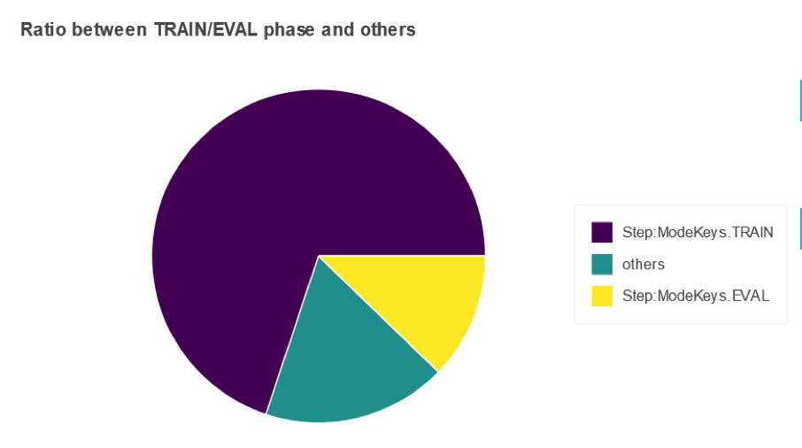
In this section of the report, you will see a pie chart similar to the below which shows how much time the training job spent in “training”, “validation” phase or “others”.
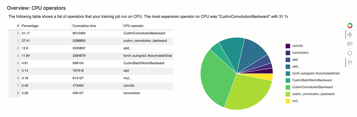
4.3 Profile Report - Identify most expensive CPU operator
Table in this section of the report shows a list of operators that your training job run on CPU. The most expensive operator on CPU was “ExecutorState::Process” with 16 %
4.4 Profile Report - Identify most expensive GPU operator
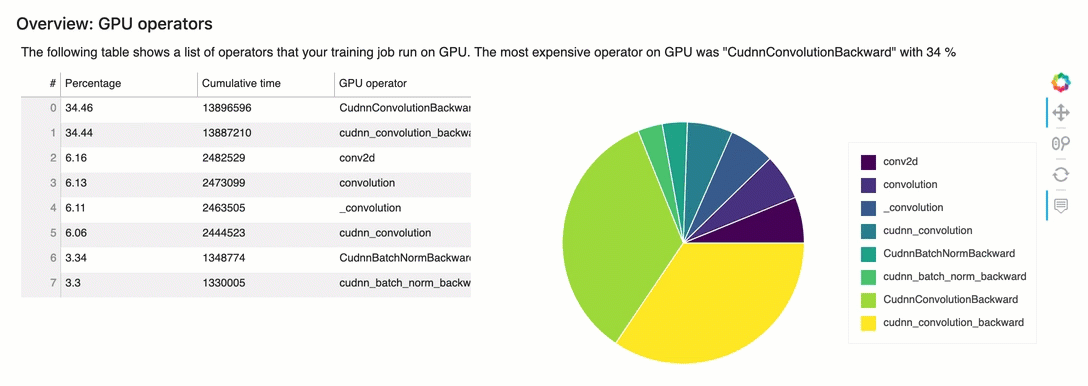
The table shows the percentage of the time and the absolute cumulative time spent on the most frequently called GPU operators.
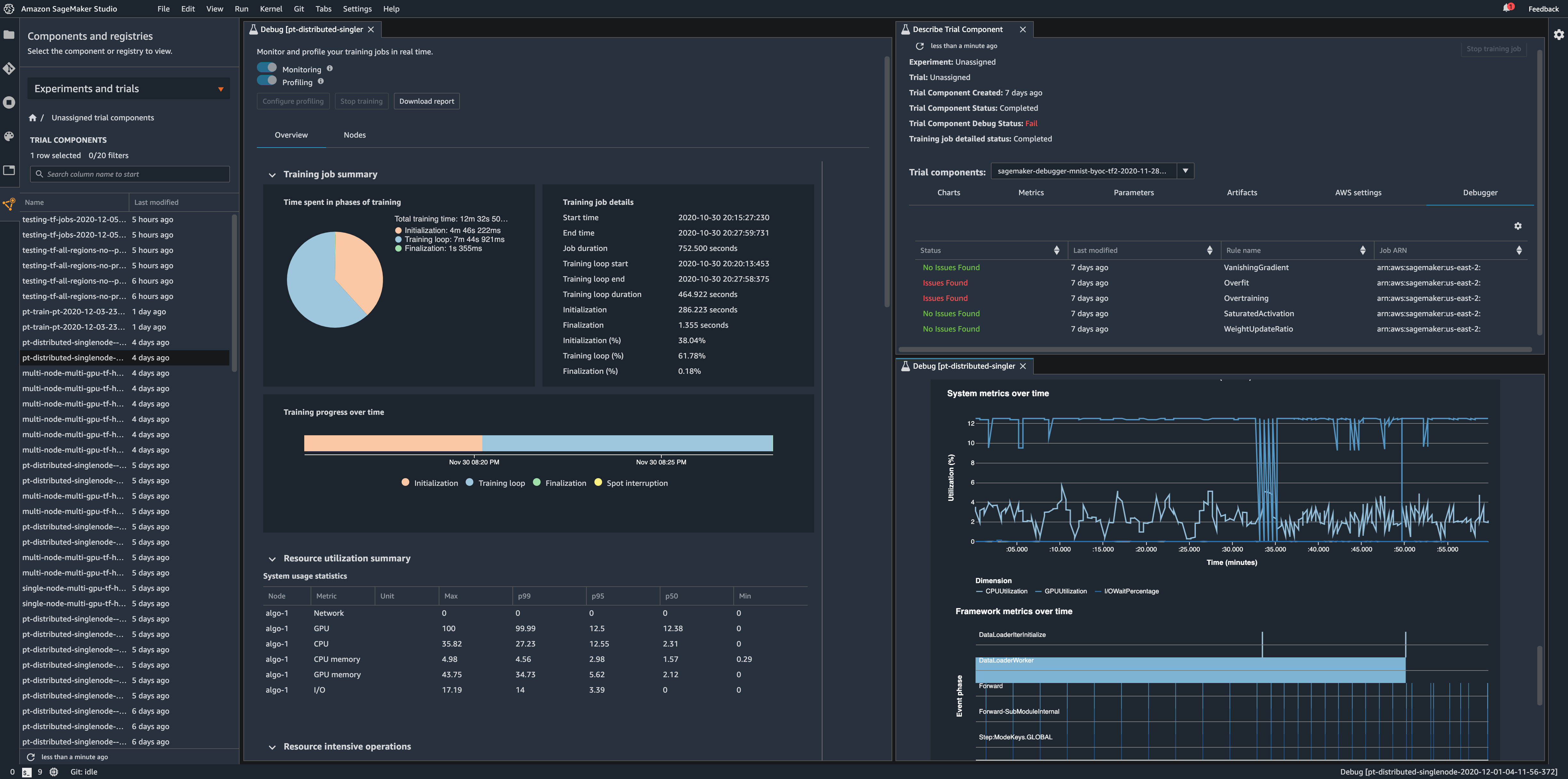
4.5 Access Debugger Insights in Amazon SageMaker Studio
In addition to interactive analysis of the Debugger output data and analyzing the autogenerated profiling report, you can also access Debugger insights dashboard from Amazon SageMaker Studio. To get started with Amazon SageMaker Studio using Debugger, see Debugger on Studio in the Amazon SageMaker Debugger developer guide.
Section 5 - Analyze recommendations from the report
The Rules Summary section of the report aggregates all of the rule evaluation results, analysis, rule descriptions, and suggestions. The following table shows a summary of the executed profiler rules. The table is sorted by the rules that triggered most frequently. In training job this was the case for rule LowGPUUtilization. It has processed 1001 datapoints and triggered 8 times.
You may see a different rule summary based on the data and the training configuration you use.
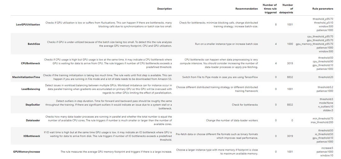
From the analysis so far and the top recommendations from the table above, there seems to be scope for improving resource utilization and make our training efficient. Based on this change the training configuration settings and re run the training.
Section 6 - Implement recommendations from the report
In the section, we will rerun the training job with the changed configuration. The training instances are changed from p3.8xlarge to p3.2xlarge instances, the number of instances is reduced to 2 and only one process per host for MPI is configured to increase the number of data loaders. The Batch Size is also changed to 512. We will use the same profiling configuration as the previous job.
After second training job with the new settings is complete, there are new system metrics, framework metrics and a new report generated.
[ ]:
hyperparameters = {"epoch": 5, "batch_size": 512, "data_augmentation": True}

distributions = {
    "mpi": {
        "enabled": True,
        "processes_per_host": 1,
        "custom_mpi_options": "-verbose -x HOROVOD_TIMELINE=./hvd_timeline.json -x NCCL_DEBUG=INFO -x OMPI_MCA_btl_vader_single_copy_mechanism=none",
    }
}

model_dir = "/opt/ml/model"
train_instance_type = "ml.p3.2xlarge"
instance_count = 2
[ ]:
estimator_new = TensorFlow(
    role=sagemaker.get_execution_role(),
    base_job_name="tf-keras-silent",
    model_dir=model_dir,
    instance_count=instance_count,
    instance_type=train_instance_type,
    entry_point="sentiment-distributed.py",
    source_dir="./tf-sentiment-script-mode",
    framework_version="2.3.1",
    py_version="py37",
    profiler_config=profiler_config,
    script_mode=True,
    hyperparameters=hyperparameters,
    distribution=distributions,
)
[ ]:
estimator_new.fit(inputs, wait=False)
Call to action
To understand the impact of the training configuration changes, compare the report analysis from the two training jobs. Repeat the process of analyzing the profiler report, implementing the recommendations and comparing with the previous run, till you are satisfied.
[ ]:
rule_output_path = (
    estimator_new.output_path + estimator_new.latest_training_job.job_name + "/rule-output"
)
print(
    f"You will find the profiler report under {rule_output_path}/ after the training has finished"
)
Download the new report and files recursively using aws s3 cp
[ ]:
! aws s3 cp {rule_output_path} ./ --recursive
Retrieve a file link to the new profiling report.
[ ]:
from IPython.display import FileLink

profiler_report_name = [
    rule["RuleConfigurationName"]
    for rule in estimator_new.latest_training_job.rule_job_summary()
    if "Profiler" in rule["RuleConfigurationName"]
][0]
profiler_report_name
display(
    "Click link below to view the profiler report",
    FileLink(profiler_report_name + "/profiler-output/profiler-report.html"),
)
Conclusion
Profiling feature of Amazon SageMaker Debugger is a powerful tool to gain visibility into machine learning training jobs. This notebook provided insight into training resource utilization to identify bottlenecks, analysis of various phases of training and identifying expensive framework functions. The notebook also demonstrated how to analyze and implement profiler recommendations. Applying profiler recommendations to a Tensorflow Horovord distributed training for a sentiment analysis model, we achieved resource utilization improvement upto 36% and up to 83% cost savings.
Notebook CI Test Results
This notebook was tested in multiple regions. The test results are as follows, except for us-west-2 which is shown at the top of the notebook.