!pip install smdebug matplotlib

Amazon SageMaker Debugger Tutorial: How to Use the Built-in Debugging Rules

---

This notebook’s CI test result for us-west-2 is as follows. CI test results in other regions can be found at the end of the notebook.

---

Amazon SageMaker Debugger is a feature that offers capability to debug training jobs of your machine learning model and identify training problems in real time. While a training job looks like it’s working like a charm, the model might have some common problems, such as loss not decreasing, overfitting, and underfitting. To better understand, practitioners have to debug the training job, while it can be challenging to track and analyze all of the output tensors.

SageMaker Debugger covers the major deep learning frameworks (TensorFlow, PyTorch, and MXNet) and machine learning algorithm (XGBoost) to do the debugging jobs with minimal coding. Debugger provides an automatic detection of training problems through its built-in rules, and you can find a full list of the built-in rules for debugging at List of Debugger Built-in Rules.

In this tutorial, you will learn how to use SageMaker Debugger and its built-in rules to debug your model.

The workflow is as follows: * Step 1: Import SageMaker Python SDK and the Debugger client library smdebug * Step 2: Create a Debugger built-in rule list object * Step 3: Construct a SageMaker estimator * Step 4: Run the training job * Step 5: Check training progress on Studio Debugger insights dashboard and the built-in rules evaluation status * Step 6: Create a Debugger trial object to access the saved tensors

## Step 1: Import SageMaker Python SDK and the SMDebug client library

Important: To use the new Debugger features, you need to upgrade the SageMaker Python SDK and the SMDebug libary. In the following cell, change the third line to install_needed=True and run to upgrade the libraries.

import sys
import IPython
install_needed = False  # Set to True to upgrade
if install_needed:
    print("installing deps and restarting kernel")
    !{sys.executable} -m pip install -U sagemaker
    !{sys.executable} -m pip install -U smdebug
    IPython.Application.instance().kernel.do_shutdown(True)

Check the SageMaker Python SDK and the SMDebug library versions.

import sagemaker

sagemaker.__version__

import smdebug

smdebug.__version__

## Step 2: Create a Debugger built-in rule list object

from sagemaker.debugger import Rule, ProfilerRule, rule_configs

The following code cell shows how to configure a rule object for debugging and profiling. For more information about the Debugger built-in rules, see List of Debugger Built-in Rules.

built_in_rules = [
    Rule.sagemaker(rule_configs.overfit()),
    ProfilerRule.sagemaker(rule_configs.ProfilerReport()),
]

## Step 3: Construct a SageMaker estimator

Using the rule object created in the previous cell, construct a SageMaker estimator.

The estimator can be one of the SageMaker framework estimators, TensorFlow, PyTorch, MXNet, and XGBoost, or the SageMaker generic estimator. For more information about what framework versions are supported, see Debugger-supported Frameworks and Algorithms.

In this tutorial, the SageMaker TensorFlow estimator is constructed to run a TensorFlow training script with the Keras ResNet50 model and the cifar10 dataset.

import boto3
from sagemaker.tensorflow import TensorFlow

session = boto3.session.Session()
region = session.region_name

estimator = TensorFlow(
    role=sagemaker.get_execution_role(),
    instance_count=1,
    instance_type="ml.p3.8xlarge",
    image_uri=f"763104351884.dkr.ecr.{region}.amazonaws.com/tensorflow-training:2.3.1-gpu-py37-cu110-ubuntu18.04",
    # framework_version='2.3.1',
    # py_version="py37",
    max_run=3600,
    source_dir="./src",
    entry_point="tf-resnet50-cifar10.py",
    # Debugger Parameters
    rules=built_in_rules,
)

## Step 4: Run the training job With the wait=False option, you can proceed to the next notebook cell without waiting for the training job logs to be printed out.

estimator.fit(wait=False)

## Step 5: Check training progress on Studio Debugger insights dashboard and the built-in rules evaluation status

• Option 1 - Use SageMaker Studio Debugger insights and Experiments. This is a non-coding approach.

• Option 2 - Use the following code cells. This is a code-based approach.

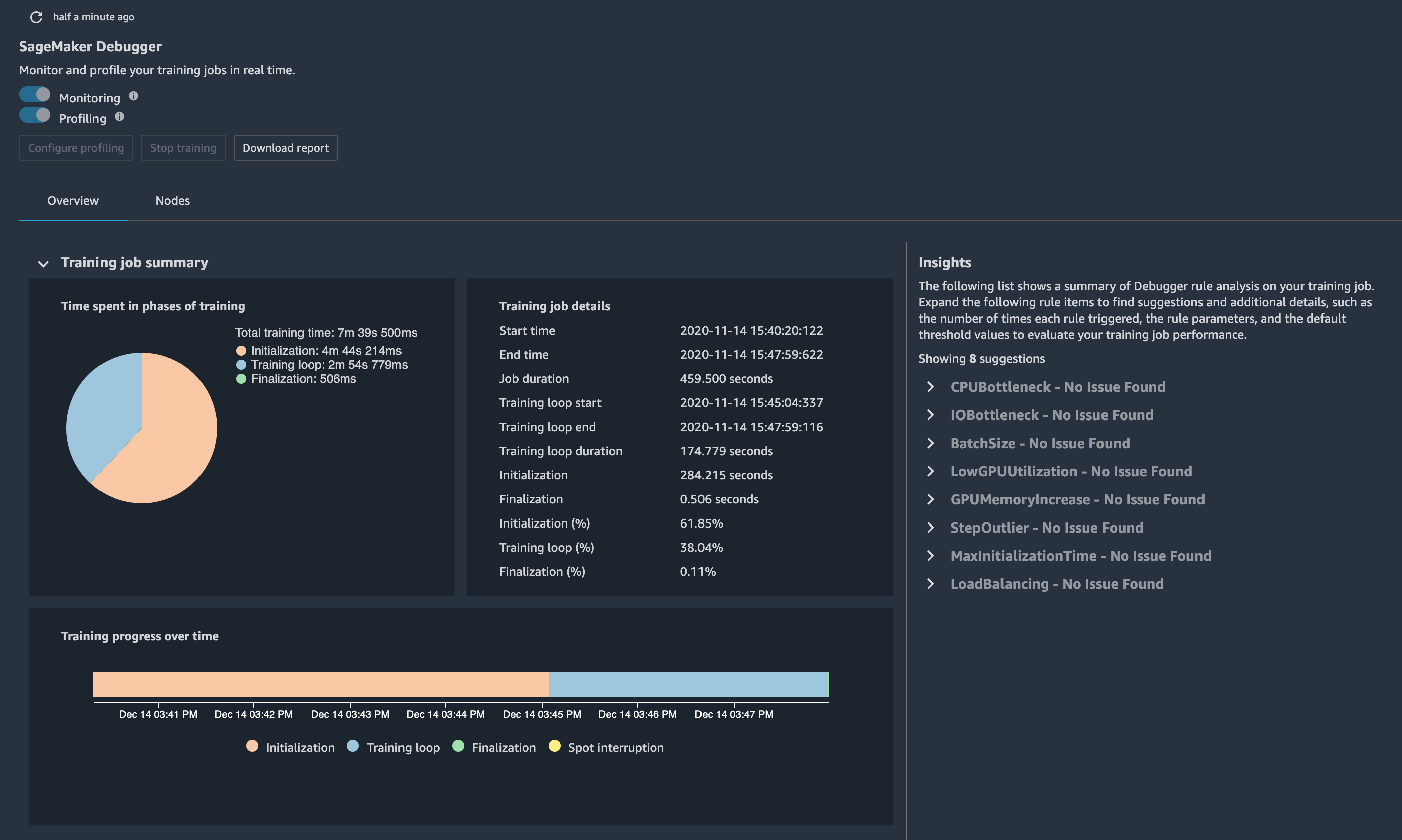
Option 1 - Open Studio Debugger insights dashboard to get insights into the training job

Through the Debugger insights dashboard on Studio, you can check the training jobs status, system resource utilization, and suggestions to optimize model performance. The following screenshot shows the Debugger insights dashboard interface.

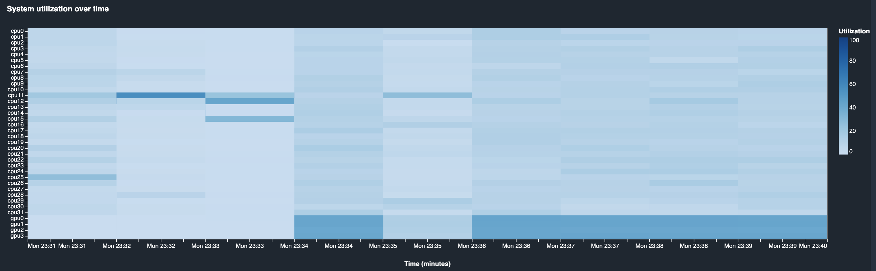
The following heatmap shows the ml.p3.8xlarge instance utilization while the training job is running or after the job has completed. To learn how to access the Debugger insights dashboard, see Debugger on Studio in the SageMaker Debugger developer guide.

Option 2 - Run the following scripts for the code-based option

The following two code cells return the current training job name, status, and the rule status in real time.

Print the training job name

job_name = estimator.latest_training_job.name
print("Training job name: {}".format(job_name))

Print the training job and rule evaluation status

The following script returns the status in real time every 15 seconds, until the secondary training status turns to one of the descriptions, Training, Stopped, Completed, or Failed. Once the training job status turns into the Training, you will be able to retrieve tensors from the default S3 bucket.

import time

client = estimator.sagemaker_session.sagemaker_client
description = client.describe_training_job(TrainingJobName=job_name)
if description["TrainingJobStatus"] != "Completed":
    while description["SecondaryStatus"] not in {"Training", "Stopped", "Completed", "Failed"}:
        description = client.describe_training_job(TrainingJobName=job_name)
        primary_status = description["TrainingJobStatus"]
        secondary_status = description["SecondaryStatus"]
        print(
            "Current job status: [PrimaryStatus: {}, SecondaryStatus: {}] | {} Rule Evaluation Status: {}".format(
                primary_status,
                secondary_status,
                estimator.latest_training_job.rule_job_summary()[0]["RuleConfigurationName"],
                estimator.latest_training_job.rule_job_summary()[0]["RuleEvaluationStatus"],
            )
        )
        time.sleep(30)

## Step 6: Create a Debugger trial object to access the saved model parameters

To access the saved tensors by Debugger, use the smdebug client library to create a Debugger trial object. The following code cell sets up a tutorial_trial object, and waits until it finds available tensors from the default S3 bucket.

from smdebug.trials import create_trial

tutorial_trial = create_trial(estimator.latest_job_debugger_artifacts_path())

The Debugger trial object accesses the SageMaker estimator’s Debugger artifact path, and fetches the output tensors saved for debugging.

Print the default S3 bucket URI where the Debugger output tensors are stored

tutorial_trial.path

Print the Debugger output tensor names

tutorial_trial.tensor_names()

Print the list of steps where the tensors are saved

The smdebug ModeKeys class provides training phase mode keys that you can use to sort training (TRAIN) and validation (EVAL) steps and their corresponding values.

from smdebug.core.modes import ModeKeys

tutorial_trial.steps(mode=ModeKeys.TRAIN)

tutorial_trial.steps(mode=ModeKeys.EVAL)

Plot the loss curve

The following script plots the loss and accuracy curves of training and validation loops.

trial = tutorial_trial


def get_data(trial, tname, mode):
    tensor = trial.tensor(tname)
    steps = tensor.steps(mode=mode)
    vals = [tensor.value(s, mode=mode) for s in steps]
    return steps, vals

import matplotlib.pyplot as plt
from mpl_toolkits.axes_grid1 import host_subplot


def plot_tensor(trial, tensor_name):
    tensor_name = tensor_name
    steps_train, vals_train = get_data(trial, tensor_name, mode=ModeKeys.TRAIN)
    steps_eval, vals_eval = get_data(trial, tensor_name, mode=ModeKeys.EVAL)

    fig = plt.figure(figsize=(10, 7))
    host = host_subplot(111)

    par = host.twiny()

    host.set_xlabel("Steps (TRAIN)")
    par.set_xlabel("Steps (EVAL)")
    host.set_ylabel(tensor_name)

    (p1,) = host.plot(steps_train, vals_train, label=tensor_name)
    (p2,) = par.plot(steps_eval, vals_eval, label="val_" + tensor_name)

    leg = plt.legend()

    host.xaxis.get_label().set_color(p1.get_color())
    leg.texts[0].set_color(p1.get_color())

    par.xaxis.get_label().set_color(p2.get_color())
    leg.texts[1].set_color(p2.get_color())

    plt.ylabel(tensor_name)

    plt.show()


plot_tensor(trial, "loss")
plot_tensor(trial, "accuracy")

Note : Rerun the above cell if you don’t see any plots!

In this tutorial, you learned how to use SageMaker Debugger with the minimal coding through SageMaker Studio and Jupyter notebook. The Debugger built-in rules detect training anomalies while concurrently reading in the output tensors, such as weights, activation outputs, gradients, accuracy, and loss, from your training jobs. In the next tutorial videos, you will learn more features of Debugger, such as how to analyze the tensors, change the built-in debugging rule parameters and thresholds, and save the tensors at your preferred S3 bucket URI.

This notebook was tested in multiple regions. The test results are as follows, except for us-west-2 which is shown at the top of the notebook.