HVAC with Amazon SageMaker RL
This notebook’s CI test result for us-west-2 is as follows. CI test results in other regions can be found at the end of the notebook.
Introduction
HVAC stands for Heating, Ventilation and Air Conditioning and is responsible for keeping us warm and comfortable indoors. HVAC takes up a whopping 50% of the energy in a building and accounts for 40% of energy use in the US [1, 2]. Several control system optimizations have been proposed to reduce energy usage while ensuring thermal comfort.
Modern buildings collect data about the weather, occupancy and equipment use. All of this can be used to optimize HVAC energy usage. Reinforcement Learning (RL) is a good fit because it can learn how to interact with the environment and identify strategies to limit wasted energy. Several recent research efforts have shown that RL can reduce HVAC energy consumption by 15-20% [3, 4].
As training an RL algorithm in a real HVAC system can take time to converge as well as potentially lead to hazardous settings as the agent explores its state space, we turn to a simulator to train the agent. EnergyPlus is an open source, state of the art HVAC simulator from the US Department of Energy. We use a simple example with this simulator to showcase how we can train an RL model easily with Amazon SageMaker RL.
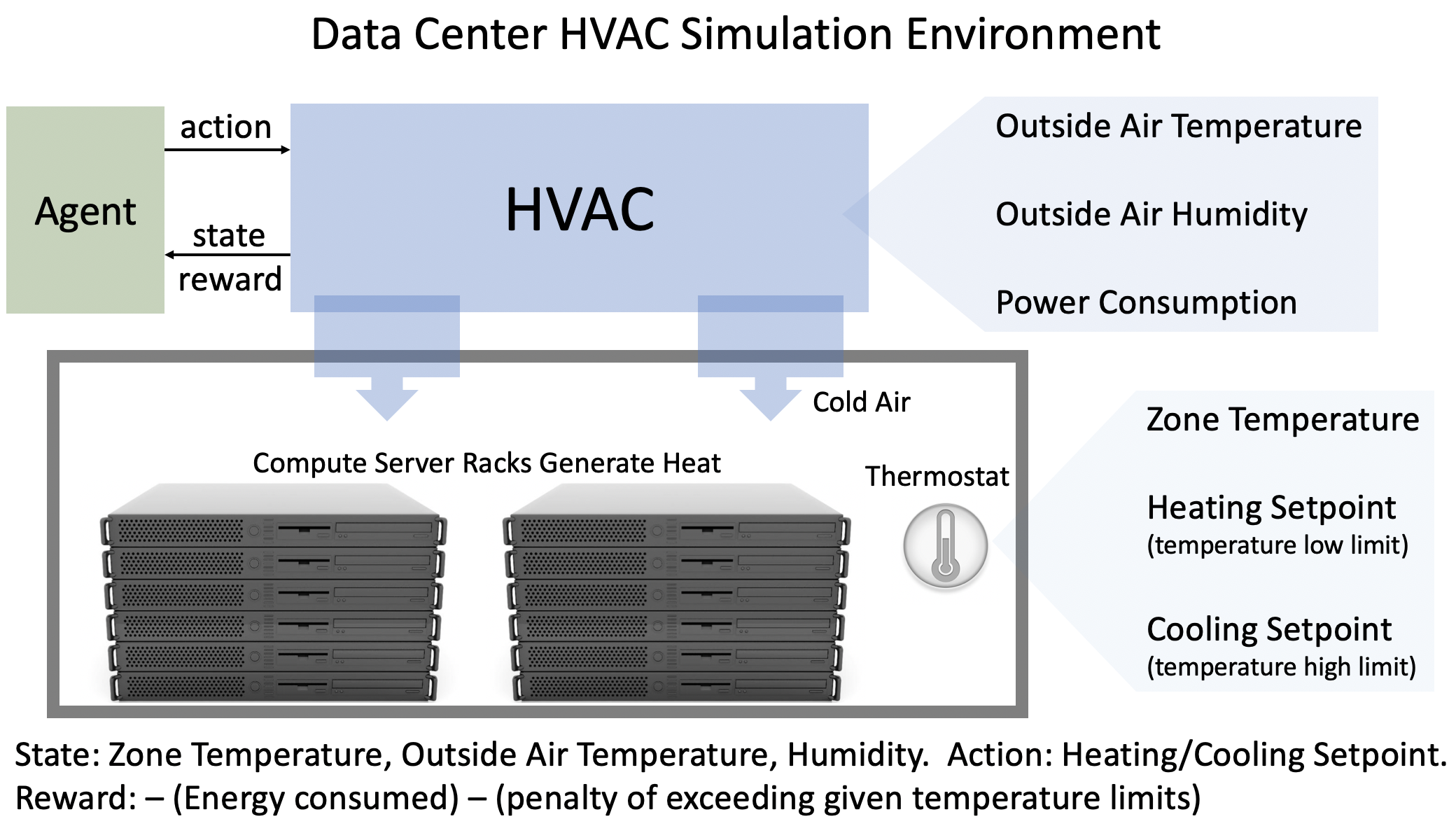
Objective: Control the data center HVAC system to reduce energy consumption while ensuring the room temperature stays within specified limits.
Environment: We have a small single room datacenter that the HVAC system is cooling to ensure the compute equipment works properly. We will train our RL agent to control this HVAC system for one day subject to weather conditions in San Francisco. The agent takes actions every 5 minutes for a 24 hour period. Hence, the episode is a fixed 120 steps.
State: The outdoor temperature, outdoor humidity and indoor room temperature.
Action: The agent can set the heating and cooling setpoints. The cooling setpoint tells the HVAC system that it should start cooling the room if the room temperature goes above this setpoint. Likewise, the HVAC systems starts heating if the room temperature goes below the heating setpoint.
Reward: The rewards has two components which are added together with coefficients:
It is proportional to the energy consumed by the HVAC system.
It gets a large penalty when the room temperature exceeds pre-specified lower or upper limits (as defined in
data_center_env.py).
References
Wei, Tianshu, Yanzhi Wang, and Qi Zhu. “Deep reinforcement learning for building hvac control.” In Proceedings of the 54th Annual Design Automation Conference 2017, p. 22. ACM, 2017.
Zhang, Zhiang, and Khee Poh Lam. “Practical implementation and evaluation of deep reinforcement learning control for a radiant heating system.” In Proceedings of the 5th Conference on Systems for Built Environments, pp. 148-157. ACM, 2018.
Pre-requisites
Imports
To get started, we’ll import the Python libraries we need, set up the environment with a few prerequisites for permissions and configurations.
[ ]:
import sagemaker
import boto3
import sys
import os
import glob
import re
import subprocess
import numpy as np
from IPython.display import HTML
import time
from time import gmtime, strftime

sys.path.append("common")
from misc import get_execution_role, wait_for_s3_object
from docker_utils import build_and_push_docker_image
from sagemaker.rl import RLEstimator, RLToolkit, RLFramework
Setup S3 bucket
Create a reference to the default S3 bucket that will be used for model outputs.
[ ]:
sage_session = sagemaker.session.Session()
s3_bucket = sage_session.default_bucket()
s3_output_path = "s3://{}/".format(s3_bucket)
print("S3 bucket path: {}".format(s3_output_path))
Define Variables
We define a job below that’s used to identify our jobs.
[ ]:
# create unique job name
job_name_prefix = "rl-hvac"
Configure settings
You can run your RL training jobs locally on the SageMaker notebook instance or on SageMaker training. In both of these scenarios, you can run in either ‘local’ (where you run the commands) or ‘SageMaker’ mode (on SageMaker training instances). ‘local’ mode uses the SageMaker Python SDK to run your code in Docker containers locally. It can speed up iterative testing and debugging while using the same familiar Python SDK interface. Just set local_mode = True. And when you’re ready move to
‘SageMaker’ mode to scale things up.
[ ]:
# run local (on this machine)?
# or on sagemaker training instances?
local_mode = False

if local_mode:
    instance_type = "local"
else:
    # choose a larger instance to avoid running out of memory
    instance_type = "ml.m4.4xlarge"
Create an IAM role
Either get the execution role when running from a SageMaker notebook instance role = sagemaker.get_execution_role() or, when running from local notebook instance, use utils method role = get_execution_role() to create an execution role.
[ ]:
try:
    role = sagemaker.get_execution_role()
except:
    role = get_execution_role()

print("Using IAM role arn: {}".format(role))
Install docker for local mode
In order to work in local mode, you need to have docker installed. When running from your local machine, please make sure that you have docker or docker-compose (for local CPU machines) and nvidia-docker (for local GPU machines) installed. Alternatively, when running from a SageMaker notebook instance, you can simply run the following script to install dependencies.
Note, you can only run a single local notebook at one time.
[ ]:
# Only run from SageMaker notebook instance
if local_mode:
    !/bin/bash ./common/setup.sh
Build docker container
Since we’re working with a custom environment with custom dependencies, we create our own container for training. We:
Fetch the base MXNet and Coach container image,
Install EnergyPlus and its dependencies on top,
Upload the new container image to AWS ECR.
[ ]:
cpu_or_gpu = "gpu" if instance_type.startswith("ml.p") else "cpu"
repository_short_name = "sagemaker-hvac-coach-%s" % cpu_or_gpu
docker_build_args = {
    "CPU_OR_GPU": cpu_or_gpu,
    "AWS_REGION": boto3.Session().region_name,
}
custom_image_name = build_and_push_docker_image(repository_short_name, build_args=docker_build_args)
print("Using ECR image %s" % custom_image_name)
Setup the environment
The environment is defined in a Python file called data_center_env.py and for SageMaker training jobs, the file will be uploaded inside the /src directory.
The environment implements the init(), step() and reset() functions that describe how the environment behaves. This is consistent with Open AI Gym interfaces for defining an environment.
init()- initialize the environment in a pre-defined statestep()- take an action on the environmentreset()- restart the environment on a new episode
Configure the presets for RL algorithm
The presets that configure the RL training jobs are defined in the “preset-energy-plus-clipped-ppo.py” file which is also uploaded as part of the /src directory. Using the preset file, you can define agent parameters to select the specific agent algorithm. You can also set the environment parameters, define the schedule and visualization parameters, and define the graph manager. The schedule presets will define the number of heat up steps, periodic evaluation steps, training steps between
evaluations, etc.
All of these can be overridden at run-time by specifying the RLCOACH_PRESET hyperparameter. Additionally, it can be used to define custom hyperparameters.
[ ]:
!pygmentize src/preset-energy-plus-clipped-ppo.py
Write the Training Code
The training code is written in the file “train-coach.py” which is uploaded in the /src directory. First import the environment files and the preset files, and then define the main() function.
[ ]:
!pygmentize src/train-coach.py
Train the RL model using the Python SDK Script mode
If you are using local mode, the training will run on the notebook instance. When using SageMaker for training, you can select a GPU or CPU instance. The RLEstimator is used for training RL jobs.
Specify the source directory where the environment, presets and training code is uploaded.
Specify the entry point as the training code
Specify the choice of RL toolkit and framework. This automatically resolves to the ECR path for the RL Container.
Define the training parameters such as the instance count, job name, S3 path for output and job name.
Specify the hyperparameters for the RL agent algorithm. The RLCOACH_PRESET can be used to specify the RL agent algorithm you want to use.
[optional] Define the metrics definitions that you are interested in capturing in your logs. These can also be visualized in CloudWatch and SageMaker Notebooks.
[ ]:
%%time
estimator = RLEstimator(
    entry_point="train-coach.py",
    source_dir="src",
    dependencies=["common/sagemaker_rl"],
    image_uri=custom_image_name,
    role=role,
    instance_type=instance_type,
    instance_count=1,
    output_path=s3_output_path,
    base_job_name=job_name_prefix,
    hyperparameters={"save_model": 1},
)

estimator.fit(wait=local_mode)
job_name = estimator.latest_training_job.job_name
print("Training job: %s" % job_name)
Store intermediate training output and model checkpoints
The output from the training job above is stored on S3. The intermediate folder contains gifs and metadata of the training.
[ ]:
s3_url = "s3://{}/{}".format(s3_bucket, job_name)

if local_mode:
    output_tar_key = "{}/output.tar.gz".format(job_name)
else:
    output_tar_key = "{}/output/output.tar.gz".format(job_name)

intermediate_folder_key = "{}/output/intermediate/".format(job_name)
output_url = "s3://{}/{}".format(s3_bucket, output_tar_key)
intermediate_url = "s3://{}/{}".format(s3_bucket, intermediate_folder_key)

print("S3 job path: {}".format(s3_url))
print("Output.tar.gz location: {}".format(output_url))
print("Intermediate folder path: {}".format(intermediate_url))

tmp_dir = "/tmp/{}".format(job_name)
os.system("mkdir {}".format(tmp_dir))
print("Create local folder {}".format(tmp_dir))
Visualization
Plot metrics for training job
We can pull the reward metric of the training and plot it to see the performance of the model over time.
[ ]:
%matplotlib inline
import pandas as pd

csv_file_name = "worker_0.simple_rl_graph.main_level.main_level.agent_0.csv"
key = os.path.join(intermediate_folder_key, csv_file_name)
wait_for_s3_object(s3_bucket, key, tmp_dir)

csv_file = "{}/{}".format(tmp_dir, csv_file_name)
df = pd.read_csv(csv_file)
df = df.dropna(subset=["Training Reward"])
x_axis = "Episode #"
y_axis = "Training Reward"

plt = df.plot(x=x_axis, y=y_axis, figsize=(12, 5), legend=True, style="b-")
plt.set_ylabel(y_axis)
plt.set_xlabel(x_axis);
Evaluation of RL models
We use the last checkpointed model to run evaluation for the RL Agent.
Load checkpointed model
Checkpointed data from the previously trained models will be passed on for evaluation / inference in the checkpoint channel. In local mode, we can simply use the local directory, whereas in the SageMaker mode, it needs to be moved to S3 first.
[ ]:
wait_for_s3_object(s3_bucket, output_tar_key, tmp_dir)

if not os.path.isfile("{}/output.tar.gz".format(tmp_dir)):
    raise FileNotFoundError("File output.tar.gz not found")
os.system("tar -xvzf {}/output.tar.gz -C {}".format(tmp_dir, tmp_dir))

if local_mode:
    checkpoint_dir = "{}/data/checkpoint".format(tmp_dir)
else:
    checkpoint_dir = "{}/checkpoint".format(tmp_dir)

print("Checkpoint directory {}".format(checkpoint_dir))
[ ]:
if local_mode:
    checkpoint_path = "file://{}".format(checkpoint_dir)
    print("Local checkpoint file path: {}".format(checkpoint_path))
else:
    checkpoint_path = "s3://{}/{}/checkpoint/".format(s3_bucket, job_name)
    if not os.listdir(checkpoint_dir):
        raise FileNotFoundError("Checkpoint files not found under the path")
    os.system("aws s3 cp --recursive {} {}".format(checkpoint_dir, checkpoint_path))
    print("S3 checkpoint file path: {}".format(checkpoint_path))
Run the evaluation step
Use the checkpointed model to run the evaluation step.
[ ]:
estimator_eval = RLEstimator(
    entry_point="evaluate-coach.py",
    source_dir="src",
    dependencies=["common/sagemaker_rl"],
    image_uri=custom_image_name,
    role=role,
    instance_type=instance_type,
    instance_count=1,
    output_path=s3_output_path,
    base_job_name=job_name_prefix + "-evaluation",
    hyperparameters={
        "RLCOACH_PRESET": "preset-energy-plus-clipped-ppo",
        "evaluate_steps": 288 * 2,  # 2 episodes, i.e. 2 days
    },
)

estimator_eval.fit({"checkpoint": checkpoint_path})
Model deployment
Since we specified MXNet when configuring the RLEstimator, the MXNet deployment container will be used for hosting.
[ ]:
from sagemaker.mxnet.model import MXNetModel

model = MXNetModel(
    model_data=estimator.model_data,
    entry_point="src/deploy-mxnet-coach.py",
    framework_version="1.8.0",
    py_version="py37",
    role=role,
)

predictor = model.deploy(initial_instance_count=1, instance_type=instance_type)
We can test the endpoint with a samples observation, where the current room temperature is high. Since the environment vector was of the form [outdoor_temperature, outdoor_humidity, indoor_humidity] and we used observation normalization in our preset, we choose an observation of [0, 0, 2]. Since we’re deploying a PPO model, our model returns both state value and actions.
[ ]:
action, action_mean, action_std = predictor.predict(
    np.array(
        [
            0.0,
            0.0,
            2.0,
        ]
    )
)
action_mean
We can see heating and cooling setpoints are returned from the model, and these can be used to control the HVAC system for efficient energy usage. More training iterations will help improve the model further.
Clean up endpoint
[ ]:
predictor.delete_endpoint()
Notebook CI Test Results
This notebook was tested in multiple regions. The test results are as follows, except for us-west-2 which is shown at the top of the notebook.