Time Series Modeling with Amazon Forecast and DeepAR on SageMaker - Amazon Forecast

This notebook’s CI test result for us-west-2 is as follows. CI test results in other regions can be found at the end of the notebook.

Introduction

Amazon offers customers a multitude of time series prediction services, including DeepAR on SageMaker and the fully managed service Amazon Forecast. Both services are similar in some aspects, yet differ in others. This notebook series aims to highlight the similarities and differences between both services by demonstrating how each service is used as well as describing the features each service offers. As a result, both notebooks in the series will use the same dataset. We will consider a real use case using the Beijing Multi-Site Air-Quality Data Set which features hourly air pollutants data from 12 air-quality monitoring sites from March 1st, 2013 to February 28th, 2017, and is featured in the [1] academic paper. This particular notebook will focus on Amazon Forecast, and will: - Explain Amazon Forecast model options - Demonstrate how to train an AutoPredictor - Create inferences from Amazon Forecast model

One feature of Amazon Forecast is that the service can be used without any code. However, this notebook will outline how to use the service within a notebook format. Before you start, please note that training an Amazon Forecast may take several hours; this particular notebook took approximately 6 hours 30 minutes to complete. Also, make sure that your SageMaker Execution Role has the following policies:

AmazonForecastFullAccess
AmazonSageMakerFullAccess
IAMFullAccess

For convenience, here is an overview of the structure of this notebook: 1. Introduction - Preparation 2. Data Preprocessing - Data Import - Data Visualization - Train/Test Split - Target/Related Time Series Split - Upload to S3 3. Dataset Group 4. Datasets - Create Datasets - Dataset Import 5. Predictors - Predictor Options - AutoPredictor 6. Forecast - Create Forecast - Query Forecast 7. Resource Cleanup 8. Next Steps

Preparation

[ ]:

!pip install seaborn --upgrade

[ ]:

import boto3
import os
import pandas as pd
import numpy as np
import json
import time
import sagemaker
from datetime import datetime
from IPython.display import display

import matplotlib.pyplot as plt
import seaborn as sns

# import forecast notebook utility library
import util

To use Amazon Forecast, we’re going to need to define an IAM role with the AmazonForecastFullAccess policy attached, as well as AmazonS3FullAccess:

[ ]:

role_name = "DemoForecastRole"
role_arn = util.get_or_create_iam_role(role_name=role_name)

[ ]:

session = boto3.Session()
s3_client = session.client("s3")
forecast_client = session.client("forecast")
forecast_query_client = session.client("forecastquery")
region = session.region_name

All paths and resource names are defined below for a simple overview for where each resource will be located:

[ ]:

# Remove paths if notebook was run before
!rm -r data
!rm -r forecast

[ ]:

bucket = sagemaker.Session().default_bucket()
sagemaker_sample_bucket = "sagemaker-sample-files"
version = datetime.now().strftime("_%Y_%m_%d_%H_%M_%S")

dirs = ["data", "forecast", "forecast/to_export"]
for dir_name in dirs:
    os.makedirs(dir_name)

dataset_s3_path = "datasets/timeseries/beijing_air_quality/PRSA2017_Data_20130301-20170228.zip"
dataset_save_path = "data/dataset.zip"  # path where the zipped dataset is imported to
dataset_path = "data/dataset"  # path where unzipped dataset is located
tts_path = "forecast/to_export/tts.csv"
rts_path = "forecast/to_export/rts.csv"
tts_s3_path = "demo-forecast/tts.csv"
rts_s3_path = "demo-forecast/rts.csv"
dataset_group_name = "demo_forecast_dsg_{}".format(version)
dataset_tts_name = "demo_forecast_tts_{}".format(version)
dataset_rts_name = "demo_forecast_rts_{}".format(version)
dataset_tts_import_name = "demo_forecast_tts_import_{}".format(version)
dataset_rts_import_name = "demo_forecast_rts_import_{}".format(version)
auto_predictor_name = "demo_forecast_auto_predictor_{}".format(version)
forecast_name = "demo_forecast_forecast_{}".format(version)

Data Preprocessing

This section prepares the dataset for use in Amazon Forecast. It will cover: - Target/Test dataset splitting - Target/Related time series splitting - S3 uploading

Data Import

This section will be demonstrating how to import data from an S3 bucket, but one can import their data whichever way is convenient. The data for this example will be imported from the sagemaker-sample-files S3 Bucket.

To communicate with S3 outside of our console, we’ll use the Boto3 python3 library. More functionality between Boto3 and S3 can be found here: Boto3 Amazon S3 Examples

This particular dataset decompresses into a single folder named PRSA_Data_20130301-20170228. It contains 12 csv files, each containing air quality data for a single location. Each DataFrame will contain the following columns: - No: row number - year: year of data in this row - month: month of data in this row - day: day of data in this row - hour: hour of data in this row - PM2.5: PM2.5 concentration (ug/m^3) - PM10: PM10 concentration (ug/m^3) - SO2: SO2 concentration (ug/m^3) - NO2: NO2 concentration (ug/m^3) - CO: CO concentration (ug/m^3) - O3: O3 concentration (ug/m^3) - TEMP: temperature (degree Celsius) - PRES: pressure (hPa) - DEWP: dew point temperature (degree Celsius) - RAIN: precipitation (mm) - wd: wind direction - WSPM: wind speed (m/s) - station: name of the air-quality monitoring site

Citations

Dua, D. and Graff, C. (2019). UCI Machine Learning Repository [http://archive.ics.uci.edu/ml]. Irvine, CA: University of California, School of Information and Computer Science.

[ ]:

s3_client.download_file(sagemaker_sample_bucket, dataset_s3_path, dataset_save_path)

[ ]:

!unzip data/dataset.zip -d data && mv data/PRSA_Data_20130301-20170228 data/dataset

[ ]:

dataset = [
    pd.read_csv("{}/{}".format(dataset_path, file_name)) for file_name in os.listdir(dataset_path)
]

display(dataset[0])

[ ]:

for df in dataset:
    df.insert(0, "datetime", pd.to_datetime(df[["year", "month", "day", "hour"]]))
    df.drop(columns=["No", "year", "month", "day", "hour"], inplace=True)

display(dataset[0])

Data Visualization

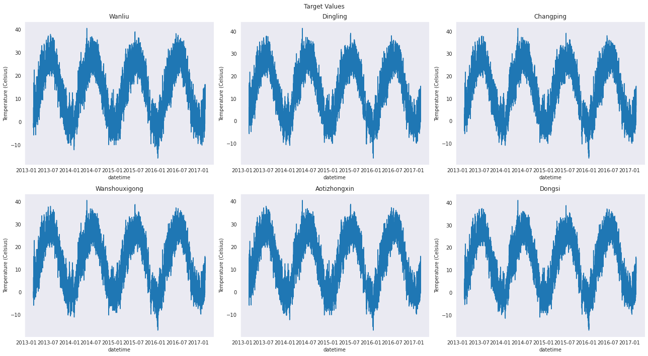
For this example, we’ll use the temperature, or TEMP column, as our target variable to predict on. Let’s first take a look at what each of our time series looks like.

[ ]:

sns.set_style("dark")
fig, axes = plt.subplots(2, 3, figsize=(18, 10))
fig.suptitle("Target Values")

for i, axis in zip(range(len(dataset))[:6], axes.ravel()):
    sns.lineplot(data=dataset[i], x="datetime", y="TEMP", ax=axis)
    axis.set_title(dataset[i]["station"].iloc[0])
    axis.set_ylabel("Temperature (Celsius)")
fig.tight_layout()

Dataset Visual

Train/Test Split

Let’s set the prediction horizon to the last 2 weeks of our time series. As a result, our test set should be the last 336 instances of each time series, as the frequency of our data is hourly.

[ ]:

prediction_length = 14 * 24

df_train = pd.concat([ts[:-prediction_length] for ts in dataset])

df_test = pd.concat([ts.tail(prediction_length) for ts in dataset])

Upload to S3

[ ]:

df_tts.to_csv(tts_path, header=False, index=False)
df_rts.to_csv(rts_path, header=False, index=False)

[ ]:

s3_client.upload_file(tts_path, bucket, tts_s3_path)
s3_client.upload_file(rts_path, bucket, rts_s3_path)

Dataset Group

A dataset group is a container for all of our resources pertaining to one particular dataset. This includes target and related time series, predictors, and forecasts.

[ ]:

response = forecast_client.create_dataset_group(
    DatasetGroupName=dataset_group_name, Domain="CUSTOM"
)

dataset_group_arn = response["DatasetGroupArn"]

Datasets

This section will go over: - Creating datasets - Creating schema - Importing datasets into dataset groups

Create Datasets

When importing datasets into Amazon Forecast, a schema for the target and/or related time series must be defined. This is a dictionary that describes the

[ ]:

display(df_tts)
display(df_rts)

[ ]:

DATASET_FREQUENCY = "H"
TIMESTAMP_FORMAT = "yyyy-MM-dd hh:mm:ss"

tts_schema = {
    "Attributes": [
        {"AttributeName": "item_id", "AttributeType": "string"},
        {"AttributeName": "timestamp", "AttributeType": "timestamp"},
        {"AttributeName": "target_value", "AttributeType": "float"},
    ]
}

response = forecast_client.create_dataset(
    Domain="CUSTOM",
    DatasetType="TARGET_TIME_SERIES",
    DatasetName=dataset_tts_name,
    DataFrequency=DATASET_FREQUENCY,
    Schema=tts_schema,
)

tts_dataset_arn = response["DatasetArn"]

[ ]:

rts_schema = {
    "Attributes": [
        {"AttributeName": "item_id", "AttributeType": "string"},
        {"AttributeName": "timestamp", "AttributeType": "timestamp"},
        {"AttributeName": "PRES", "AttributeType": "float"},
        {"AttributeName": "RAIN", "AttributeType": "float"},
        {"AttributeName": "WSPM", "AttributeType": "float"},
    ]
}

response = forecast_client.create_dataset(
    Domain="CUSTOM",
    DatasetType="RELATED_TIME_SERIES",
    DatasetName=dataset_rts_name,
    DataFrequency=DATASET_FREQUENCY,
    Schema=rts_schema,
)

rts_dataset_arn = response["DatasetArn"]

[ ]:

forecast_client.update_dataset_group(
    DatasetGroupArn=dataset_group_arn,
    DatasetArns=[
        tts_dataset_arn,
        rts_dataset_arn,
    ],
)

Dataset Import

[ ]:

response = forecast_client.create_dataset_import_job(
    DatasetImportJobName=dataset_tts_import_name,
    DatasetArn=tts_dataset_arn,
    DataSource={
        "S3Config": {"Path": "s3://{}/{}".format(bucket, tts_s3_path), "RoleArn": role_arn}
    },
    TimestampFormat=TIMESTAMP_FORMAT,
)

tts_dataset_import_job_arn = response["DatasetImportJobArn"]

[ ]:

response = forecast_client.create_dataset_import_job(
    DatasetImportJobName=dataset_tts_import_name,
    DatasetArn=rts_dataset_arn,
    DataSource={
        "S3Config": {"Path": "s3://{}/{}".format(bucket, rts_s3_path), "RoleArn": role_arn}
    },
    TimestampFormat=TIMESTAMP_FORMAT,
)

rts_dataset_import_job_arn = response["DatasetImportJobArn"]

[ ]:

while True:
    tts_status = forecast_client.describe_dataset_import_job(
        DatasetImportJobArn=tts_dataset_import_job_arn
    )["Status"]
    rts_status = forecast_client.describe_dataset_import_job(
        DatasetImportJobArn=rts_dataset_import_job_arn
    )["Status"]
    if tts_status == "ACTIVE" and rts_status == "ACTIVE":
        break
    if tts_status == "CREATE_FAILED" or rts_status == "CREATE_FAILED":
        print("Dataset Import Job Failed")
        break
    time.sleep(10)

Predictors

Predictor Options

Amazon Forecast offers six built-in algorithms: 1. CNN-QR 2. DeepAR+ 3. Prophet 4. NPTS 5. ARIMA 6. ETS

Optimal use cases for each algorithm can be found here: Comparing Forecast Algorithms

In addition to multiple algorithms, Amazon Forecast offers three options for predictions: - Manual Selection - Manually select a single algorithm to apply to entire dataset - AutoML - Service finds and applies best-performing algorithm to entire dataset - AutoPredictor - Service runs all models and blends predictions with the goal of improving accuracy

Manual selection and AutoML are considered Legacy models, and new features will only be supported by the AutoPredictor model. As a result, the AutoPredictor model will be used in this notebook. More information on Amazon Forecast’s AutoPredictor can be found here: Amazon Forecast AutoPredictor

AutoPredictor

This particular auto-predictor took approximately 6 hours 17 minutes to train.

[ ]:

response = forecast_client.create_auto_predictor(
    PredictorName=auto_predictor_name,
    ForecastHorizon=prediction_length,
    ForecastFrequency=DATASET_FREQUENCY,
    DataConfig={"DatasetGroupArn": dataset_group_arn},
)

auto_predictor_arn = response["PredictorArn"]

[ ]:

util.wait(lambda: forecast_client.describe_auto_predictor(PredictorArn=auto_predictor_arn))

Forecast

Create Forecast

[ ]:

response = forecast_client.create_forecast(
    ForecastName=forecast_name, PredictorArn=auto_predictor_arn
)

forecast_arn = response["ForecastArn"]

[ ]:

while True:
    status = forecast_client.describe_forecast(ForecastArn=forecast_arn)["Status"]
    if status in ("ACTIVE", "CREATE_FAILED"):
        break
    time.sleep(10)

Query Forecast

[ ]:

def plot_comparison(item_id):

    response = forecast_query_client.query_forecast(
        ForecastArn=forecast_arn, Filters={"item_id": item_id}
    )

    def query_to_df(query):
        predictions = query["Forecast"]["Predictions"]
        dfs = []
        for quantile in predictions:
            temp = pd.DataFrame.from_dict(predictions[quantile]).rename(
                columns={"Timestamp": "datetime", "Value": quantile}
            )
            temp["datetime"] = pd.to_datetime(temp["datetime"]).dt.tz_localize(None)
            dfs.append(temp)
        return pd.concat(dfs, axis=1).T.drop_duplicates().T

    query = query_to_df(response)

    plt.figure(figsize=(18, 10))
    plt.plot(query["datetime"], query["p10"], color="r", lw=1)
    plt.plot(query["datetime"], query["p50"], color="orange", linestyle=":", lw=2)
    plt.plot(query["datetime"], query["p90"], color="r", lw=1)
    plt.plot(
        query["datetime"], df_tts_test[df_tts_test["station"] == item_id]["TEMP"], color="b", lw=1
    )
    plt.fill_between(
        query["datetime"].tolist(),
        query["p90"].tolist(),
        query["p10"].tolist(),
        color="y",
        alpha=0.5,
    )

    plt.title(item_id)
    plt.xlabel("Datetime")
    plt.ylabel("Temperature (Celsius)")

    plt.legend(["10% Quantile", "50% Quantile", "90% Quantile", "Target"])
    plt.show()

[ ]:

stations = df_tts_test["station"].unique()
plot_comparison(stations[0])

Forecast Results

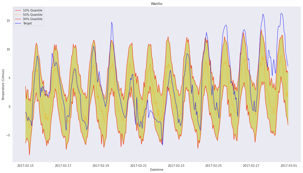
The plot above shows the target values and 10%, 50%, and 90% quantiles. The 10% and 90% quantiles produce an 80% confidence interval.

Resource Cleanup

Let’s clean up every resource we’ve created throughout this notebook. We’ll have to delete our resources in a specific order: 1. Delete Forecasts 2. Delete Predictors 3. Delete Dataset Imports 4. Delete Datasets 5. Delete Dataset Group 6. Delete IAM Role

[ ]:

util.wait_till_delete(lambda: forecast_client.delete_forecast(ForecastArn=forecast_arn))

[ ]:

util.wait_till_delete(lambda: forecast_client.delete_predictor(PredictorArn=auto_predictor_arn))

[ ]:

util.wait_till_delete(
    lambda: forecast_client.delete_dataset_import_job(
        DatasetImportJobArn=tts_dataset_import_job_arn
    )
)
util.wait_till_delete(
    lambda: forecast_client.delete_dataset_import_job(
        DatasetImportJobArn=rts_dataset_import_job_arn
    )
)

[ ]:

util.wait_till_delete(lambda: forecast_client.delete_dataset(DatasetArn=tts_dataset_arn))
util.wait_till_delete(lambda: forecast_client.delete_dataset(DatasetArn=rts_dataset_arn))

[ ]:

util.wait_till_delete(
    lambda: forecast_client.delete_dataset_group(DatasetGroupArn=dataset_group_arn)
)

[ ]:

util.delete_iam_role(role_name)

Next Steps

This notebook illustrates the features offered by Amazon Forecast, and is part of the Time Series Modeling with Amazon Forecast and DeepAR on SageMaker series. The notebook series aims to demonstrate how to use the Amazon Forecast and DeepAR on SageMaker time series modeling services as well as outline their features. Be sure to read the DeepAR on SageMaker example, and view a top-level comparison of both services in the README.

Notebook CI Test Results

This notebook was tested in multiple regions. The test results are as follows, except for us-west-2 which is shown at the top of the notebook.