Train and Host a Keras Model with Pipe Mode and Horovod on Amazon SageMaker
This notebook’s CI test result for us-west-2 is as follows. CI test results in other regions can be found at the end of the notebook.
Amazon SageMaker is a fully-managed service that provides developers and data scientists with the ability to build, train, and deploy machine learning (ML) models quickly. Amazon SageMaker removes the heavy lifting from each step of the machine learning process to make it easier to develop high-quality models. The SageMaker Python SDK makes it easy to train and deploy models in Amazon SageMaker with several different machine learning and deep learning frameworks, including TensorFlow and Keras.
In this notebook, we train and host a Keras Sequential model on SageMaker. The model used for this notebook is a simple deep convolutional neural network (CNN) that was extracted from the Keras examples.
For training our model, we also demonstrate distributed training with Horovod and Pipe Mode. Amazon SageMaker’s Pipe Mode streams your dataset directly to your training instances instead of being downloaded first, which translates to training jobs that start sooner, finish quicker, and need less disk space.
Setup
First, we define a few variables that are be needed later in the example.
[ ]:
import sagemaker
from sagemaker import get_execution_role

sagemaker_session = sagemaker.Session()

role = get_execution_role()
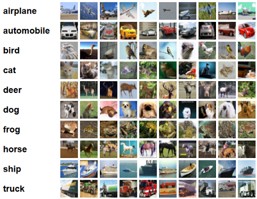
The CIFAR-10 dataset
The CIFAR-10 dataset is one of the most popular machine learning datasets. It consists of 60,000 32x32 images belonging to 10 different classes (6,000 images per class). Here are the classes in the dataset, as well as 10 random images from each:
Prepare the dataset for training
To use the CIFAR-10 dataset, we first download it and convert it to TFRecords. This step takes around 5 minutes.
[ ]:
!python generate_cifar10_tfrecords.py --data-dir ./data
Next, we upload the data to Amazon S3:
[ ]:
from sagemaker.s3 import S3Uploader

bucket = sagemaker_session.default_bucket()
dataset_uri = S3Uploader.upload("data", "s3://{}/tf-cifar10-example/data".format(bucket))

display(dataset_uri)
Train the model
In this tutorial, we train a deep CNN to learn a classification task with the CIFAR-10 dataset. We compare three different training jobs: a baseline training job, training with Pipe Mode, and distributed training with Horovod.
Run a baseline training job on SageMaker
The SageMaker Python SDK’s sagemaker.tensorflow.TensorFlow estimator class makes it easy for us to interact with SageMaker. We create one for each of the different training jobs we run in this example. A couple parameters worth noting:
entry_point: our training script (adapted from this Keras example).train_instance_count: the number of training instances. Here, we set it to 1 for our baseline training job.
As we run each of our training jobs, we change different parameters to configure our different training jobs.
For more details about the TensorFlow estimator class, see the API documentation.
Verify the training code
Before running the baseline training job, we first use the SageMaker Python SDK’s Local Mode feature to check that our code works with SageMaker’s TensorFlow environment. Local Mode downloads the prebuilt Docker image for TensorFlow and runs a Docker container locally for a training job. In other words, it simulates the SageMaker environment for a quicker development cycle, so we use it here just to test out our code.
We create a TensorFlow estimator, and specify the instance_type to be 'local' or 'local_gpu', depending on our local instance type. This tells the estimator to run our training job locally (as opposed to on SageMaker). We also have our training code run for only one epoch because our intent here is to verify the code, not train an accurate model.
[ ]:
import subprocess

from sagemaker.tensorflow import TensorFlow

instance_type = "local"

if subprocess.call("nvidia-smi") == 0:
    # Set instance type to GPU if one is present
    instance_type = "local_gpu"

local_hyperparameters = {"epochs": 1, "batch-size": 64}

estimator = TensorFlow(
    entry_point="cifar10_keras_main.py",
    source_dir="source_dir",
    role=role,
    framework_version="1.15.2",
    py_version="py3",
    hyperparameters=local_hyperparameters,
    train_instance_count=1,
    train_instance_type=instance_type,
)
Once we have our estimator, we call fit() to start the training job and pass the inputs that we downloaded earlier. We pass the inputs as a dictionary to define different data channels for training.
[ ]:
import os

data_path = os.path.join(os.getcwd(), "data")

local_inputs = {
    "train": "file://{}/train".format(data_path),
    "validation": "file://{}/validation".format(data_path),
    "eval": "file://{}/eval".format(data_path),
}
estimator.fit(local_inputs)
Run a baseline training job on SageMaker
Now we run training jobs on SageMaker, starting with our baseline training job.
Configure metrics
In addition to running the training job, Amazon SageMaker can retrieve training metrics directly from the logs and send them to CloudWatch metrics. Here, we define metrics we would like to observe:
[ ]:
metric_definitions = [
    {"Name": "train:loss", "Regex": ".*loss: ([0-9\\.]+) - accuracy: [0-9\\.]+.*"},
    {"Name": "train:accuracy", "Regex": ".*loss: [0-9\\.]+ - accuracy: ([0-9\\.]+).*"},
    {
        "Name": "validation:accuracy",
        "Regex": ".*step - loss: [0-9\\.]+ - accuracy: [0-9\\.]+ - val_loss: [0-9\\.]+ - val_accuracy: ([0-9\\.]+).*",
    },
    {
        "Name": "validation:loss",
        "Regex": ".*step - loss: [0-9\\.]+ - accuracy: [0-9\\.]+ - val_loss: ([0-9\\.]+) - val_accuracy: [0-9\\.]+.*",
    },
    {
        "Name": "sec/steps",
        "Regex": ".* - \d+s (\d+)[mu]s/step - loss: [0-9\\.]+ - accuracy: [0-9\\.]+ - val_loss: [0-9\\.]+ - val_accuracy: [0-9\\.]+",
    },
]
Once again, we create a TensorFlow estimator, with a couple key modfications from last time:
train_instance_type: the instance type for training. We set this toml.p2.xlargebecause we are training on SageMaker now. For a list of available instance types, see the AWS documentation.metric_definitions: the metrics (defined above) that we want sent to CloudWatch.
[ ]:
from sagemaker.tensorflow import TensorFlow

hyperparameters = {"epochs": 10, "batch-size": 256}
tags = [{"Key": "Project", "Value": "cifar10"}, {"Key": "TensorBoard", "Value": "file"}]

estimator = TensorFlow(
    entry_point="cifar10_keras_main.py",
    source_dir="source_dir",
    metric_definitions=metric_definitions,
    hyperparameters=hyperparameters,
    role=role,
    framework_version="1.15.2",
    py_version="py3",
    train_instance_count=1,
    train_instance_type="ml.p2.xlarge",
    base_job_name="cifar10-tf",
    tags=tags,
)
Like before, we call fit() to start the SageMaker training job and pass the inputs in a dictionary to define different data channels for training. This time, we use the S3 URI from uploading our data.
[ ]:
inputs = {
    "train": "{}/train".format(dataset_uri),
    "validation": "{}/validation".format(dataset_uri),
    "eval": "{}/eval".format(dataset_uri),
}

estimator.fit(inputs)
View the job training metrics
We can now view the metrics from the training job directly in the SageMaker console.
Log into the SageMaker console, choose the latest training job, and scroll down to the monitor section. Alternatively, the code below uses the region and training job name to generate a URL to CloudWatch metrics.
Using CloudWatch metrics, you can change the period and configure the statistics.
[ ]:
from urllib import parse

from IPython.core.display import Markdown

region = sagemaker_session.boto_region_name
cw_url = parse.urlunparse(
    (
        "https",
        "{}.console.aws.amazon.com".format(region),
        "/cloudwatch/home",
        "",
        "region={}".format(region),
        "metricsV2:namespace=/aws/sagemaker/TrainingJobs;dimensions=TrainingJobName;search={}".format(
            estimator.latest_training_job.name
        ),
    )
)

display(
    Markdown(
        "CloudWatch metrics: [link]({}). After you choose a metric, "
        "change the period to 1 Minute (Graphed Metrics -> Period).".format(cw_url)
    )
)
Train on SageMaker with Pipe Mode
Here we train our model using Pipe Mode. With Pipe Mode, SageMaker uses Linux named pipes to stream the training data directly from S3 instead of downloading the data first.
In our script, we enable Pipe Mode using the following code:
from sagemaker_tensorflow import PipeModeDataset

dataset = PipeModeDataset(channel=channel_name, record_format='TFRecord')
When we create our estimator, the only difference from before is that we also specify input_mode='Pipe':
[ ]:
pipe_mode_estimator = TensorFlow(
    entry_point="cifar10_keras_main.py",
    source_dir="source_dir",
    metric_definitions=metric_definitions,
    hyperparameters=hyperparameters,
    role=role,
    framework_version="1.15.2",
    py_version="py3",
    train_instance_count=1,
    train_instance_type="ml.p2.xlarge",
    input_mode="Pipe",
    base_job_name="cifar10-tf-pipe",
    tags=tags,
)
In this example, we set wait=False if you want to see the output logs, change this to wait=True
[ ]:
pipe_mode_estimator.fit(inputs, wait=False)
Distributed training with Horovod
Horovod is a distributed training framework based on MPI. To use Horovod, we make the following changes to our training script:
Enable Horovod:
import horovod.keras as hvd

hvd.init()
config = tf.ConfigProto()
config.gpu_options.allow_growth = True
config.gpu_options.visible_device_list = str(hvd.local_rank())
K.set_session(tf.Session(config=config))
Add these callbacks:
hvd.callbacks.BroadcastGlobalVariablesCallback(0)
hvd.callbacks.MetricAverageCallback()
Configure the optimizer:
opt = Adam(lr=learning_rate * size, decay=weight_decay)
opt = hvd.DistributedOptimizer(opt)
Choose to save checkpoints and send TensorBoard logs only from the master node:
if hvd.rank() == 0:
    save_model(model, args.model_output_dir)
To configure the training job, we specify the following for the distribution:
[ ]:
distribution = {
    "mpi": {
        "enabled": True,
        "processes_per_host": 1,  # Number of Horovod processes per host
    }
}
This is then passed to our estimator, in addition to setting train_instance_count to 2:
[ ]:
dist_estimator = TensorFlow(
    entry_point="cifar10_keras_main.py",
    source_dir="source_dir",
    metric_definitions=metric_definitions,
    hyperparameters=hyperparameters,
    distributions=distribution,
    role=role,
    framework_version="1.15.2",
    py_version="py3",
    train_instance_count=2,
    train_instance_type="ml.p3.2xlarge",
    base_job_name="cifar10-tf-dist",
    tags=tags,
)
Like before, we call fit() on our estimator. If you want to see the training job logs in the notebook output, set wait=True.
[ ]:
dist_estimator.fit(inputs, wait=False)
Compare the training jobs with TensorBoard
Using the visualization tool TensorBoard, we can compare our training jobs.
In a local setting, install TensorBoard with pip install tensorboard. Then run the command generated by the following code:
[ ]:
!python generate_tensorboard_command.py
After running that command, we can access TensorBoard locally at http://localhost:6006.
Based on the TensorBoard metrics, we can see that: 1. All jobs run for 10 epochs (0 - 9). 1. Both File Mode and Pipe Mode run for ~1 minute - Pipe Mode doesn’t affect training performance. 1. Distributed training runs for only 45 seconds. 1. All of the training jobs resulted in similar validation accuracy.
This example uses a relatively small dataset (179 MB). For larger datasets, Pipe Mode can significantly reduce training time because it does not copy the entire dataset into local memory.
Deploy the trained model
After we train our model, we can deploy it to a SageMaker Endpoint, which serves prediction requests in real-time. To do so, we simply call deploy() on our estimator, passing in the desired number of instances and instance type for the endpoint.
Because we’re using TensorFlow Serving for deployment, our training script saves the model in TensorFlow’s SavedModel format. For more details, see this blog post on deploying Keras and TF models in SageMaker.
[ ]:
predictor = estimator.deploy(initial_instance_count=1, instance_type="ml.m4.xlarge")
Invoke the endpoint
To verify the that the endpoint is in service, we generate some random data in the correct shape and get a prediction.
[ ]:
import numpy as np

data = np.random.randn(1, 32, 32, 3)
print("Predicted class: {}".format(np.argmax(predictor.predict(data)["predictions"])))
Now let’s use the test dataset for predictions.
[ ]:
from keras.datasets import cifar10

(x_train, y_train), (x_test, y_test) = cifar10.load_data()
With the data loaded, we can use it for predictions:
[ ]:
from keras.preprocessing.image import ImageDataGenerator


def predict(data):
    predictions = predictor.predict(data)["predictions"]
    return predictions


predicted = []
actual = []
batches = 0
batch_size = 128

datagen = ImageDataGenerator()
for data in datagen.flow(x_test, y_test, batch_size=batch_size):
    for i, prediction in enumerate(predict(data[0])):
        predicted.append(np.argmax(prediction))
        actual.append(data[1][i][0])

    batches += 1
    if batches >= len(x_test) / batch_size:
        break
With the predictions, we calculate our model accuracy and create a confusion matrix.
[ ]:
from sklearn.metrics import accuracy_score

accuracy = accuracy_score(y_pred=predicted, y_true=actual)
display("Average accuracy: {}%".format(round(accuracy * 100, 2)))
[ ]:
%matplotlib inline
import matplotlib.pyplot as plt
import pandas as pd
import seaborn as sn
from sklearn.metrics import confusion_matrix

cm = confusion_matrix(y_pred=predicted, y_true=actual)
cm = cm.astype("float") / cm.sum(axis=1)[:, np.newaxis]
sn.set(rc={"figure.figsize": (11.7, 8.27)})
sn.set(font_scale=1.4)  # for label size
sn.heatmap(cm, annot=True, annot_kws={"size": 10})  # font size
Aided by the colors of the heatmap, we can use this confusion matrix to understand how well the model performed for each label.
Cleanup
To avoid incurring extra charges to your AWS account, let’s delete the endpoint we created:
[ ]:
predictor.delete_endpoint()
Notebook CI Test Results
This notebook was tested in multiple regions. The test results are as follows, except for us-west-2 which is shown at the top of the notebook.