Using SageMaker Debugger and SageMaker Experiments for iterative model pruning
This notebook’s CI test result for us-west-2 is as follows. CI test results in other regions can be found at the end of the notebook.
This notebook demonstrates how we can use SageMaker Debugger and SageMaker Experiments to perform iterative model pruning. Let’s start first with a quick introduction into model pruning.
State-of-the-art deep learning models consist of millions of parameters and are trained on very large datasets. For transfer learning we take a pre-trained model and fine-tune it on a new and typically much smaller dataset. The new dataset may even consist of different classes, so the model is basically learning a new task. This process allows us to quickly achieve state-of-the-artresults without having to design and train our own model from scratch. However, it may happen that a much smaller and simpler model would also perform well on our dataset. With model pruning we identify the importance of weights during training and remove the weights that are contributing very little to the learning process. We can do this in an iterative way where we remove a small percentage of weights in each iteration. Removing means to eliminate the entries in the tensor so its size shrinks.
We use SageMaker Debugger to get weights, activation outputs and gradients during training. These tensors are used to compute the importance of weights. We will use SageMaker Experiments to keep track of each pruning iteration: if we prune too much we may degrade model accuracy, so we will monitor number of parameters versus validation accuracy.
[ ]:
import pip
import sys

def import_or_install(package):
    try:
        __import__(package)
    except ImportError:
        !{sys.executable} -m pip install {package}

required_packages=['smdebug', 'sagemaker-experiments']
Get training dataset
Next we get the Caltech-101 dataset. This dataset consists of 101 image categories.
[ ]:
import tarfile
import requests
import os

filename = "101_ObjectCategories.tar.gz"
data_url = os.path.join("https://s3.us-east-2.amazonaws.com/mxnet-public", filename)

r = requests.get(data_url, stream=True)
with open(filename, "wb") as f:
    for chunk in r.iter_content(chunk_size=1024):
        if chunk:
            f.write(chunk)

print("Extracting {} ...".format(filename))
tar = tarfile.open(filename, "r:gz")
tar.extractall(".")
tar.close()
print("Data extracted.")
And upload it to our SageMaker default bucket:
[ ]:
import sagemaker
import boto3


def upload_to_s3(path, directory_name, bucket, counter=-1):
    print("Upload files from" + path + " to " + bucket)
    client = boto3.client("s3")

    for path, subdirs, files in os.walk(path):
        path = path.replace("\\", "/")
        print(path)
        for file in files[0:counter]:
            client.upload_file(
                os.path.join(path, file),
                bucket,
                directory_name + "/" + path.split("/")[-1] + "/" + file,
            )


boto_session = boto3.Session()
sagemaker_session = sagemaker.Session(boto_session=boto_session)
bucket = sagemaker_session.default_bucket()

upload_to_s3("101_ObjectCategories", directory_name="101_ObjectCategories_train", bucket=bucket)

# we will compute saliency maps for all images in the test dataset, so we will only upload 4 images
upload_to_s3(
    "101_ObjectCategories_test",
    directory_name="101_ObjectCategories_test",
    bucket=bucket,
    counter=4,
)
Load and save ResNet model
First we load a pre-trained ResNet model from PyTorch model zoo.
[ ]:
import torch
from torchvision import models
from torch import nn

model = models.resnet18(pretrained=True)
Let’s have a look on the model architecture:
[ ]:
model
As we can see above, the last Linear layer outputs 1000 values, which is the number of classes the model has originally been trained on. Here, we will fine-tune the model on the Caltech101 dataset: as it has only 101 classes, we need to set the number of output classes to 101.
[ ]:
nfeatures = model.fc.in_features
model.fc = torch.nn.Linear(nfeatures, 101)
Next we store the model definition and weights in an output file.
IMPORTANT: the model file will be used by the training job. To avoid version conflicts, you need to ensure that your notebook is running a Jupyter kernel with PyTorch version 1.6.
[ ]:
checkpoint = {"model": model, "state_dict": model.state_dict()}

torch.save(checkpoint, "src/model_checkpoint")
The following code cell creates a SageMaker experiment:
[ ]:
import boto3
from datetime import datetime
from smexperiments.experiment import Experiment

sagemaker_boto_client = boto3.client("sagemaker")

# name of experiment
timestep = datetime.now()
timestep = timestep.strftime("%d-%m-%Y-%H-%M-%S")
experiment_name = timestep + "resnet-model-pruning-experiment"

# create experiment
Experiment.create(
    experiment_name=experiment_name,
    description="Iterative model pruning of ResNet trained on Caltech101",
    sagemaker_boto_client=sagemaker_boto_client,
)
The following code cell defines a list of tensor names that be used to compute filter ranks. The lists are defined in the Python script model_resnet.
[ ]:
import model_resnet

activation_outputs = model_resnet.activation_outputs
gradients = model_resnet.gradients
Iterative model pruning: step by step
Before we jump into the code for running the iterative model pruning we will walk through the code step by step.
Step 0: Create trial and debugger hook configuration
First we create a new trial for each pruning iteration. That allows us to track our training jobs and see which models have the lowest number of parameters and best accuracy. We use the smexperiments library to create a trial within our experiment.
[ ]:
from smexperiments.trial import Trial

trial = Trial.create(experiment_name=experiment_name, sagemaker_boto_client=sagemaker_boto_client)
Next we define the experiment_config which is a dictionary that will be passed to the SageMaker training.
[ ]:
experiment_config = {
    "ExperimentName": experiment_name,
    "TrialName": trial.trial_name,
    "TrialComponentDisplayName": "Training",
}
We create a debugger hook configuration to define a custom collection of tensors to be emitted. The custom collection contains all weights and biases of the model. It also includes individual layer outputs and their gradients which will be used to compute filter ranks. Tensors are saved every 100th iteration where an iteration represents one forward and backward pass.
[ ]:
from sagemaker.debugger import DebuggerHookConfig, CollectionConfig

debugger_hook_config = DebuggerHookConfig(
    collection_configs=[
        CollectionConfig(
            name="custom_collection",
            parameters={
                "include_regex": ".*relu|.*weight|.*bias|.*running_mean|.*running_var|.*CrossEntropyLoss",
                "save_interval": "100",
            },
        )
    ]
)
Step 1: Start training job
Now we define the SageMaker PyTorch Estimator. We will train the model on an ml.p2.xlarge instance. The model definition plus training code is defined in the entry_point file train.py.
[ ]:
import sagemaker
from sagemaker.pytorch import PyTorch

estimator = PyTorch(
    role=sagemaker.get_execution_role(),
    instance_count=1,
    instance_type="ml.p3.2xlarge",
    volume_size=400,
    source_dir="src",
    entry_point="train.py",
    framework_version="1.12",
    py_version="py38",
    metric_definitions=[
        {"Name": "train:loss", "Regex": "loss:(.*?)"},
        {"Name": "eval:acc", "Regex": "acc:(.*?)"},
    ],
    enable_sagemaker_metrics=True,
    hyperparameters={"epochs": 10},
    debugger_hook_config=debugger_hook_config,
)
After we define the estimator object, we can call fit which creates an ml.p2.xlarge instance on which it starts the training. We pass the experiment_config which associates the training job with a trial and an experiment. If we don’t specify an experiment_config, the training job will appear in SageMaker Experiments under Unassigned trial components.
[ ]:
estimator.fit(
    inputs={
        "train": "s3://{}/101_ObjectCategories_train".format(bucket),
        "test": "s3://{}/101_ObjectCategories_test".format(bucket),
    },
    experiment_config=experiment_config,
)
Step 2: Get gradients, weights, biases
Once the training job has finished, we will retrieve its tensors, such as gradients, weights and biases. We use the smdebug library which provides functions to read and filter tensors. First we create a trial that is reading the tensors from S3.
For clarification: in the context of SageMaker Debugger a trial is an object that lets you query tensors for a given training job. In the context of SageMaker Experiments a trial is part of an experiment; it presents a collection of training steps involved in a single training job.
[ ]:
from smdebug.trials import create_trial

path = estimator.latest_job_debugger_artifacts_path()
smdebug_trial = create_trial(path)
To access tensor values, we only need to call smdebug_trial.tensor(). For instance, to get the outputs of the first ReLU activation at step 0, we run smdebug_trial.tensor('layer4.1.relu_0_output_0').value(0, mode=modes.TRAIN). Next we compute a filter rank for the convolutions.
Some definitions: a filter is a collection of kernels (one kernel for every single input channel) and a filter produces one feature map (output channel). In the image below the convolution creates 64 feature maps (output channels) and uses a kernel of 5x5. By pruning a filter, an entire feature map will be removed. So in the example image below the number of feature maps (output channels) would shrink to 63 and the number of learnable parameters (weights) would be reduced by 1x5x5.
Step 3: Compute filter ranks
In this notebook we compute filter ranks as described in the article “Pruning Convolutional Neural Networks for Resource Efficient Inference” We basically identify filters that are less important for the final prediction of the model. The product of weights and gradients can be seen as a measure of importance. The product has the dimension (batch_size, out_channels, width, height) and we get the average over axis=0,2,3 to have a single value
(rank) for each filter.
In the following code we retrieve activation outputs and gradients and compute the filter rank.
[ ]:
import numpy as np
from smdebug import modes


def compute_filter_ranks(smdebug_trial, activation_outputs, gradients):
    filters = {}
    for activation_output_name, gradient_name in zip(activation_outputs, gradients):
        for step in smdebug_trial.steps(mode=modes.TRAIN):
            activation_output = smdebug_trial.tensor(activation_output_name).value(
                step, mode=modes.TRAIN
            )
            gradient = smdebug_trial.tensor(gradient_name).value(step, mode=modes.TRAIN)
            rank = activation_output * gradient
            rank = np.mean(rank, axis=(0, 2, 3))

            if activation_output_name not in filters:
                filters[activation_output_name] = 0
            filters[activation_output_name] += rank
    return filters


filters = compute_filter_ranks(smdebug_trial, activation_outputs, gradients)
Next we normalize the filters:
[ ]:
def normalize_filter_ranks(filters):
    for activation_output_name in filters:
        rank = np.abs(filters[activation_output_name])
        rank = rank / np.sqrt(np.sum(rank * rank))
        filters[activation_output_name] = rank
    return filters


filters = normalize_filter_ranks(filters)
We create a list of filters, sort it by rank and retrieve the smallest values:
[ ]:
def get_smallest_filters(filters, n):
    filters_list = []
    for layer_name in sorted(filters.keys()):
        for channel in range(filters[layer_name].shape[0]):
            filters_list.append(
                (
                    layer_name,
                    channel,
                    filters[layer_name][channel],
                )
            )

    filters_list.sort(key=lambda x: x[2])
    filters_list = filters_list[:n]
    print("The", n, "smallest filters", filters_list)

    return filters_list


filters_list = get_smallest_filters(filters, 100)
Step 4 and step 5: Prune low ranking filters and set new weights
Next we prune the model, where we remove filters and their corresponding weights.
[ ]:
step = smdebug_trial.steps(mode=modes.TRAIN)[-1]

model = model_resnet.prune(model, filters_list, smdebug_trial, step)
Step 6: Start next pruning iteration
Once we have pruned the model, the new architecture and pruned weights will be saved under src and will be used by the next training job in the next pruning iteration.
[ ]:
# save pruned model
checkpoint = {"model": model, "state_dict": model.state_dict()}

torch.save(checkpoint, "src/model_checkpoint")

# clean up
del model
Overall workflow
The overall workflow looks like the following:
Run iterative model pruning
After having gone through the code step by step, we are ready to run the full workflow. The following cell runs 1 pruning iteration for a tutorial purpose. Change the range of the for loop to 10 to replicate the same result shown in the Pruning machine learning models with Amazon SageMaker Debugger and Amazon SageMaker Experiments blog and the figure below the cell. In each iteration a new SageMaker training job is started, where it emits gradients and activation outputs to Amazon S3. Once the job has finished, filter ranks are computed and the 100 smallest filters are removed.
[ ]:
# start iterative pruning
for pruning_step in range(1):
    # create new trial for this pruning step
    smexperiments_trial = Trial.create(
        experiment_name=experiment_name, sagemaker_boto_client=sagemaker_boto_client
    )
    experiment_config["TrialName"] = smexperiments_trial.trial_name

    print("Created new trial", smexperiments_trial.trial_name, "for pruning step", pruning_step)

    # start training job
    estimator = PyTorch(
        role=sagemaker.get_execution_role(),
        instance_count=1,
        instance_type="ml.p3.2xlarge",
        volume_size=400,
        source_dir="src",
        entry_point="train.py",
        framework_version="1.6",
        py_version="py3",
        metric_definitions=[
            {"Name": "train:loss", "Regex": "loss:(.*?)"},
            {"Name": "eval:acc", "Regex": "acc:(.*?)"},
        ],
        enable_sagemaker_metrics=True,
        hyperparameters={"epochs": 10},
        debugger_hook_config=debugger_hook_config,
    )

    # start training job
    estimator.fit(
        inputs={
            "train": "s3://{}/101_ObjectCategories_train".format(bucket),
            "test": "s3://{}/101_ObjectCategories_test".format(bucket),
        },
        experiment_config=experiment_config,
    )

    print("Training job", estimator.latest_training_job.name, " finished.")

    # read tensors
    path = estimator.latest_job_debugger_artifacts_path()
    smdebug_trial = create_trial(path)

    # compute filter ranks and get 100 smallest filters
    filters = compute_filter_ranks(smdebug_trial, activation_outputs, gradients)
    filters_normalized = normalize_filter_ranks(filters)
    filters_list = get_smallest_filters(filters_normalized, 100)

    # load previous model
    checkpoint = torch.load("src/model_checkpoint")
    model = checkpoint["model"]
    model.load_state_dict(checkpoint["state_dict"])

    # prune model
    step = smdebug_trial.steps(mode=modes.TRAIN)[-1]
    model = model_resnet.prune(model, filters_list, smdebug_trial, step)

    print("Saving pruned model")

    # save pruned model
    checkpoint = {"model": model, "state_dict": model.state_dict()}
    torch.save(checkpoint, "src/model_checkpoint")

    # clean up
    del model
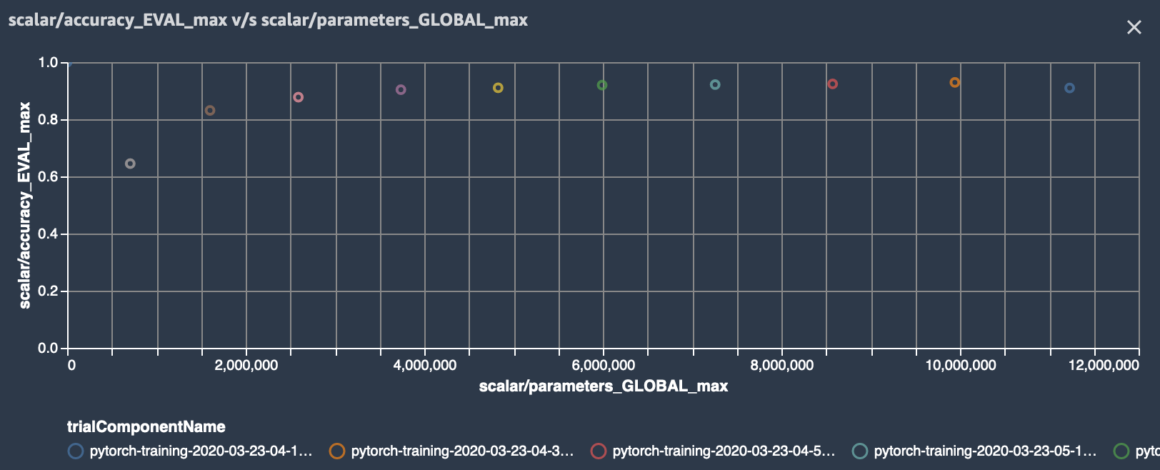
As the iterative model pruning is running, we can track and visualize our experiment in SageMaker Studio. In our training script we use SageMaker debugger’s save_scalar method to store the number of parameters in the model and the model accuracy. So we can visualize those in Studio or use the ExperimentAnalytics module to read and plot the values directly in the notebook.
Initially the model consisted of 11 million parameters. After 11 iterations, the number of parameters was reduced to 270k, while accuracy increased to 91% and then started dropping after 8 pruning iteration.
This means that the best accuracy can be reached if the model has a size of about 4 million parameters, while shrinking model size about 3x!
Additional: run iterative model pruning with custom rule
In the previous example, we have seen that accuracy drops when the model has less than 22 million parameters. Clearly, we want to stop our experiment once we reach this point. We can define a custom rule that returns True if the accuracy drops by a certain percentage. You can find an example implementation in custom_rule/check_accuracy.py. Before we can use the rule we have to define a custom rule configuration:
from sagemaker.debugger import Rule, CollectionConfig, rule_configs

check_accuracy_rule = Rule.custom(
    name='CheckAccuracy',
    image_uri='759209512951.dkr.ecr.us-west-2.amazonaws.com/sagemaker-debugger-rule-evaluator:latest',
    instance_type='ml.c4.xlarge',
    volume_size_in_gb=400,
    source='custom_rule/check_accuracy.py',
    rule_to_invoke='check_accuracy',
    rule_parameters={"previous_accuracy": "0.0",
                     "threshold": "0.05",
                     "predictions": "CrossEntropyLoss_0_input_0",
                     "labels":"CrossEntropyLoss_0_input_1"},
)
The rule reads the inputs to the loss function, which are the model predictions and the labels. It computes the accuracy and returns True if its value has dropped by more than 5% otherwise False.
In each pruning iteration, we need to pass the accuracy of the previous training job to the rule, which can be retrieved via the ExperimentAnalytics module.
from sagemaker.analytics import ExperimentAnalytics

trial_component_analytics = ExperimentAnalytics(experiment_name=experiment_name)
accuracy = trial_component_analytics.dataframe()['scalar/accuracy_EVAL - Max'][0]
And overwrite the value in the rule configuration:
check_accuracy_rule.rule_parameters["previous_accuracy"] = str(accuracy)
In the PyTorch estimator we need to add the argument rules = [check_accuracy_rule]. We can create a CloudWatch alarm and use a Lambda function to stop the training. Detailed instructions can be found here. In each iteration we check the job status and if the previous job has been stopped, we exit the loop:
job_name = estimator.latest_training_job.name
client = estimator.sagemaker_session.sagemaker_client
description = client.describe_training_job(TrainingJobName=job_name)

if description['TrainingJobStatus'] == 'Stopped':
      break
Notebook CI Test Results
This notebook was tested in multiple regions. The test results are as follows, except for us-west-2 which is shown at the top of the notebook.