Using SageMaker debugger to monitor autoencoder model training

---

This notebook’s CI test result for us-west-2 is as follows. CI test results in other regions can be found at the end of the notebook.

---

This notebook will train a convolutional autoencoder model on MNIST dataset and use SageMaker debugger to monitor key metrics in realtime. An autoencoder consists of an encoder that downsamples input data and a decoder that tries to reconstruct the original input. In this notebook we will use an autoencoder with the following architecture:

--------------------------------------------------------------------------------
        Layer (type)                                Output Shape         Param #
================================================================================
               Input                              (1, 1, 28, 28)               0
        Activation-1  <Symbol hybridsequential0_conv0_relu_fwd>                0
        Activation-2                             (1, 32, 24, 24)               0
            Conv2D-3                             (1, 32, 24, 24)             832
         MaxPool2D-4                             (1, 32, 12, 12)               0
        Activation-5  <Symbol hybridsequential0_conv1_relu_fwd>                0
        Activation-6                               (1, 32, 8, 8)               0
            Conv2D-7                               (1, 32, 8, 8)           25632
         MaxPool2D-8                               (1, 32, 4, 4)               0
             Dense-9                                     (1, 20)           10260
       Activation-10  <Symbol hybridsequential1_dense0_relu_fwd>               0
       Activation-11                                    (1, 512)               0
            Dense-12                                    (1, 512)           10752
     HybridLambda-13                               (1, 32, 8, 8)               0
       Activation-14  <Symbol hybridsequential1_conv0_relu_fwd>                0
       Activation-15                             (1, 32, 12, 12)               0
  Conv2DTranspose-16                             (1, 32, 12, 12)           25632
     HybridLambda-17                             (1, 32, 24, 24)               0
       Activation-18  <Symbol hybridsequential1_conv1_sigmoid_fwd>             0
       Activation-19                              (1, 1, 28, 28)               0
  Conv2DTranspose-20                              (1, 1, 28, 28)             801
ConvolutionalAutoencoder-21                       (1, 1, 28, 28)               0
================================================================================
Parameters in forward computation graph, duplicate included
   Total params: 73909
   Trainable params: 73909
   Non-trainable params: 0
Shared params in forward computation graph: 0
Unique parameters in model: 73909
--------------------------------------------------------------------------------

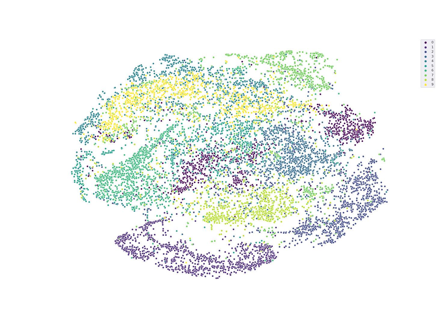
The bottleneck layer forces the autoencoder to learn a compressed representation (latent variables) of the dataset. Visualizing the latent space helps to understand what the autoencoder is learning. We can check if the model is training well by checking - reconstructed images (autoencoder output) - t-Distributed Stochastic Neighbor Embedding (t-SNE) of the latent variables

t-SNE maps high dimensional data into a 2- or 3-dimensional space. Following animation shows those emebeddings of latent variables while the training progresses. Each cluster represents a class (0-9) of the MNIST training dataset. Over time the autoencoder becomes better in separating those classes.

Training MXNet autoencoder model in Amazon SageMaker with debugger

Before starting the SageMaker training job, we need to install some libraries. We will use smdebug library to read, filter and analyze raw tensors that are stored in Amazon S3. We install seaborn library that will be used later on to plot t-Distributed Stochastic Neighbor Embedding (t-SNE) of the latent variables.

import pip


def import_or_install(package):
    try:
        __import__(package)
    except ImportError:
        ! pip install $package

import_or_install("smdebug")

import_or_install("seaborn")

First we define the MXNet estimator and the debugger hook configuration. The model training is implemented in the entry point script autoencoder_mnist.py. We will obtain tensors every 10th iteration and store them in the SageMaker default bucket.

import sagemaker
from sagemaker.mxnet import MXNet
from sagemaker.debugger import DebuggerHookConfig, CollectionConfig

sagemaker_session = sagemaker.Session()
BUCKET_NAME = sagemaker_session.default_bucket()
LOCATION_IN_BUCKET = "smdebug-autoencoder-example"

s3_bucket_for_tensors = "s3://{BUCKET_NAME}/{LOCATION_IN_BUCKET}".format(
    BUCKET_NAME=BUCKET_NAME, LOCATION_IN_BUCKET=LOCATION_IN_BUCKET
)
estimator = MXNet(
    role=sagemaker.get_execution_role(),
    base_job_name="mxnet",
    train_instance_count=1,
    train_instance_type="ml.m5.xlarge",
    train_volume_size=400,
    source_dir="src",
    entry_point="autoencoder_mnist.py",
    framework_version="1.6.0",
    py_version="py3",
    debugger_hook_config=DebuggerHookConfig(
        s3_output_path=s3_bucket_for_tensors,
        collection_configs=[
            CollectionConfig(
                name="all",
                parameters={
                    "include_regex": ".*convolutionalautoencoder0_hybridsequential0_dense0_output_0|.*convolutionalautoencoder0_input_1|.*loss",
                    "save_interval": "10",
                },
            )
        ],
    ),
)

Start the training job:

estimator.fit(wait=False)

We can check the S3 location of tensors:

path = estimator.latest_job_debugger_artifacts_path()
print("Tensors are stored in: {}".format(path))

Get the training job name:

job_name = estimator.latest_training_job.name
print("Training job name: {}".format(job_name))

client = estimator.sagemaker_session.sagemaker_client

description = client.describe_training_job(TrainingJobName=job_name)

We can access the tensors from S3 once the training job is in status Training or Completed. In the following code cell we check the job status.

import time

if description["TrainingJobStatus"] != "Completed":
    while description["SecondaryStatus"] not in {"Training", "Completed"}:
        description = client.describe_training_job(TrainingJobName=job_name)
        primary_status = description["TrainingJobStatus"]
        secondary_status = description["SecondaryStatus"]
        print(
            "Current job status: [PrimaryStatus: {}, SecondaryStatus: {}]".format(
                primary_status, secondary_status
            )
        )
        time.sleep(15)

Get tensors and visualize model training in real-time

In this section, we will retrieve the tensors from the bottlneck layer and input/output tensors while the model is still training. Once we have the tensors, we will compute t-SNE and plot the results.

Helper function to compute stochastic neighbor embeddings:

from sklearn.manifold import TSNE


def compute_tsne(tensors, labels):
    # compute TSNE
    tsne = TSNE(n_components=2, verbose=1, perplexity=40, n_iter=300)
    tsne_results = tsne.fit_transform(tensors)

    # add results to dictionary
    data = {}
    data["x"] = tsne_results[:, 0]
    data["y"] = tsne_results[:, 1]
    data["z"] = labels

    return data

Helper function to plot t-SNE results and autoencoder input/output.

import matplotlib.pyplot as plt
import seaborn as sns


def plot_autoencoder_data(tsne_results, input_tensor, output_tensor):
    fig, (ax0, ax1, ax2) = plt.subplots(
        ncols=3, figsize=(30, 15), gridspec_kw={"width_ratios": [1, 1, 3]}
    )
    plt.rcParams.update({"font.size": 20})
    ax0.imshow(input_tensor, cmap=plt.cm.gray)
    ax1.imshow(output_tensor, cmap=plt.cm.gray)
    ax0.set_axis_off()
    ax1.set_axis_off()
    ax2.set_axis_off()
    ax0.set_title("autoencoder input")
    ax1.set_title("autoencoder output")
    plt.title("Step " + str(step))
    sns.scatterplot(
        x="x", y="y", hue="z", data=tsne_results, palette="viridis", legend="full", s=100
    )
    plt.legend(bbox_to_anchor=(1.05, 1), loc=2, borderaxespad=0.0)
    plt.axis("off")
    plt.show()
    plt.clf()

Create trial:

from smdebug.trials import create_trial

trial = create_trial(estimator.latest_job_debugger_artifacts_path())

Get available steps

steps = 0
while steps == 0:
    steps = trial.steps()
    print("Waiting for tensors to become available...")
    time.sleep(3)
print("\nDone")

print("Getting tensors...")
rendered_steps = []

To determine how well the autoencoder is training, we will get the following tensors: - Dense layer: we will compute the t-distributed stochastic neighbor embeddings (t-SNE) of the tensors retrieved from the bottleneck layer. - Input label: will be used to mark the embeddigns. Emebeddings with the same label should be in the same clsuter. - Autoencoder input and output: to determine the reconstruction performance of the autoencoder.

label_input = "convolutionalautoencoder0_input_1"
autoencoder_bottleneck = "convolutionalautoencoder0_hybridsequential0_dense0_output_0"
autoencoder_input = "l2loss0_input_1"
autoencoder_output = "l2loss0_input_0"

Following code cell iterates over available steps, retrieves the tensors and computes t-SNE.

from smdebug.exceptions import TensorUnavailableForStep
from smdebug.mxnet import modes

loaded_all_steps = False
while not loaded_all_steps:
    # get available steps
    loaded_all_steps = trial.loaded_all_steps
    steps = trial.steps(mode=modes.EVAL)

    # quick way to get diff between two lists
    steps_to_render = list(set(steps).symmetric_difference(set(rendered_steps)))

    tensors = []
    labels = []

    # iterate over available steps
    for step in sorted(steps_to_render):
        try:
            if len(tensors) > 1000:
                tensors = []
                labels = []

            # get tensor from bottleneck layer and label
            tensor = trial.tensor(autoencoder_bottleneck).value(step_num=step, mode=modes.EVAL)
            label = trial.tensor(label_input).value(step_num=step, mode=modes.EVAL)
            for batch in range(tensor.shape[0]):
                tensors.append(tensor[batch, :])
                labels.append(label[batch])

            # compute tsne
            tsne_results = compute_tsne(tensors, labels)

            # get autoencoder input and output
            input_tensor = trial.tensor(autoencoder_input).value(step_num=step, mode=modes.EVAL)[
                0, 0, :, :
            ]
            output_tensor = trial.tensor(autoencoder_output).value(step_num=step, mode=modes.EVAL)[
                0, 0, :, :
            ]

            # plot results
            plot_autoencoder_data(tsne_results, input_tensor, output_tensor)

        except TensorUnavailableForStep:
            print("Tensor unavilable for step {}".format(step))

    rendered_steps.extend(steps_to_render)

    time.sleep(5)

print("\nDone")

Notebook CI Test Results

This notebook was tested in multiple regions. The test results are as follows, except for us-west-2 which is shown at the top of the notebook.