---

This notebook’s CI test result for us-west-2 is as follows. CI test results in other regions can be found at the end of the notebook.

---

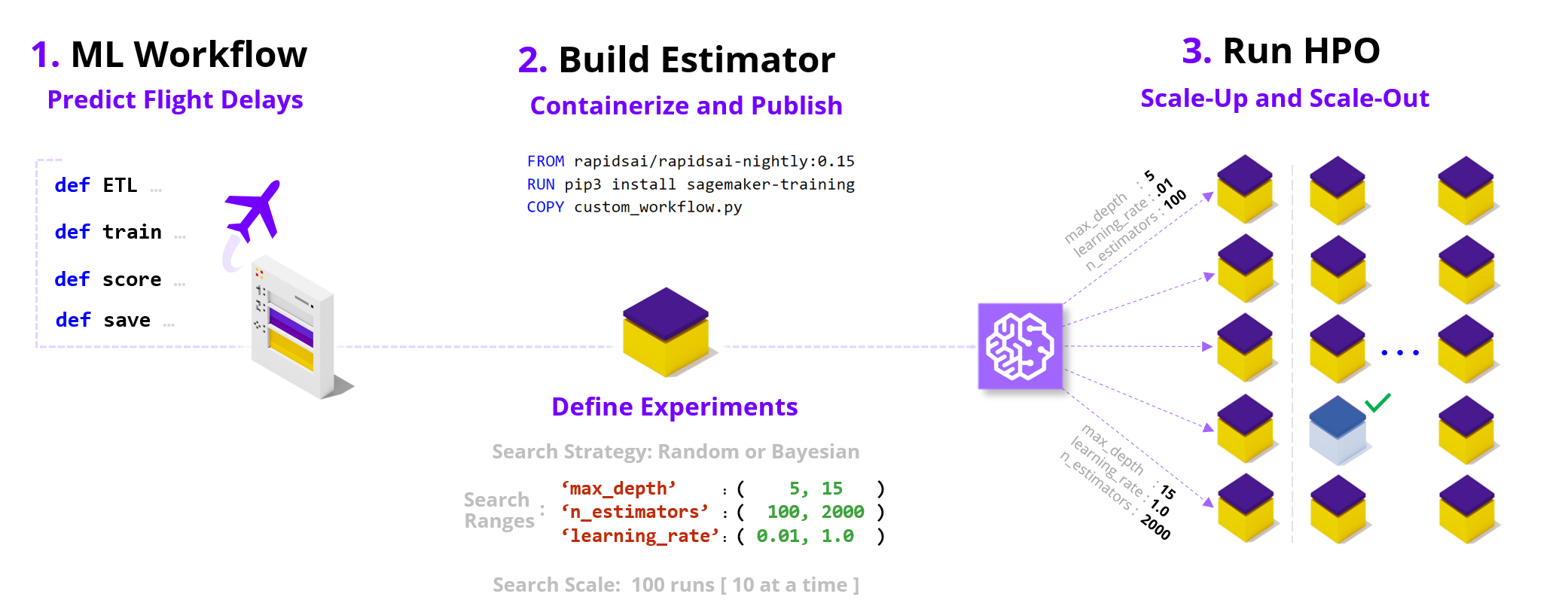
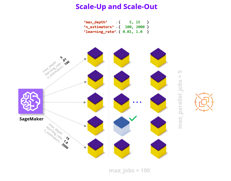
Hyper Parameter Optimization (HPO) improves model quality by searching over hyperparameters, parameters not typically learned during the training process but rather values that control the learning process itself (e.g., model size/capacity). This search can significantly boost model quality relative to default settings and non-expert tuning; however, HPO can take a very long time on a non-accelerated platform. In this notebook, we containerize a RAPIDS workflow and run Bring-Your-Own-Container SageMaker HPO to show how we can overcome the computational complexity of model search.

We accelerate HPO in two key ways: * by scaling within a node (e.g., multi-GPU where each GPU brings a magnitude higher core count relative to CPUs), and * by scaling across nodes and running parallel trials on cloud instances.

By combining these two powers HPO experiments that feel unapproachable and may take multiple days on CPU instances can complete in just hours. For example, we find a 12x speedup in wall clock time (6 hours vs 3+ days) and a 4.5x reduction in cost when comparing between GPU and CPU EC2 Spot instances on 100 XGBoost HPO trials using 10 parallel workers on 10 years of the Airline Dataset (~63M flights) hosted in a S3 bucket. For additional details refer to the end of the notebook.

With all these powerful tools at our disposal, every data scientist should feel empowered to up-level their model before serving it to the world!

Preamble

To get things rolling let’s make sure we can query our AWS SageMaker execution role and session as well as our account ID and AWS region.

import sagemaker
from helper_functions import *

execution_role = sagemaker.get_execution_role()
session = sagemaker.Session()

account=!(aws sts get-caller-identity --query Account --output text)
region=!(aws configure get region)

account, region

Key Choices

Let’s go ahead and choose the configuration options for our HPO run.

Below are two reference configurations showing a small and a large scale HPO (sized in terms of total experiments/compute).

The default values in the notebook are set for the small HPO configuration, however you are welcome to scale them up.

small HPO: 1_year, XGBoost, 3 CV folds, singleGPU, max_jobs = 10, max_parallel_jobs = 2

large HPO: 10_year, XGBoost, 10 CV folds, multiGPU, max_jobs = 100, max_parallel_jobs = 10

[ Dataset ]

We offer free hosting for several demo datasets that you can try running HPO with, or alternatively you can bring your own dataset (BYOD).

By default we leverage the Airline dataset, which is a large public tracker of US domestic flight logs which we offer in various sizes (1 year, 3 year, and 10 year) and in Parquet (compressed column storage) format. The machine learning objective with this dataset is to predict whether flights will be more than 15 minutes late arriving to their destination (dataset link, additional details in Section 1.1).

As an alternative we also offer the NYC Taxi dataset which captures yellow cab trip details in Ney York in January 2020, stored in CSV format without any compression. The machine learning objective with this dataset is to predict whether a trip had an above average tip (>$2.20).

We host the demo datasets in public S3 demo buckets in both the us-east-1 (N. Virginia) or us-west-2 (Oregon) regions (i.e., sagemaker-rapids-hpo-us-east-1, and sagemaker-rapids-hpo-us-west-2). You should run the SageMaker HPO workflow in either of these two regions if you wish to leverage the demo datasets since SageMaker requires that the S3 dataset and the compute you’ll be renting are co-located.

Lastly, if you plan to use your own dataset refer to the BYOD checklist in the Appendix to help integrate into the workflow.

dataset	data_bucket	dataset_directory	# samples	storage type	time span
Airline Stats Small	demo	1_year	6.3M	Parquet	2019
Airline Stats Medium	demo	3_year	18M	Parquet	2019-2017
Airline Stats Large	demo	10_year	63M	Parquet	2019-2010
NYC Taxi	demo	NYC_taxi	6.3M	CSV	2020 January
Bring Your Own Dataset	custom	custom	custom	Parquet/CSV	custom

# please choose dataset S3 bucket and directory
data_bucket = "sagemaker-rapids-hpo-" + region[0]
dataset_directory = "3_year"  # '3_year', '10_year', 'NYC_taxi'

# please choose output bucket for trained model(s)
model_output_bucket = session.default_bucket()

s3_data_input = f"s3://{data_bucket}/{dataset_directory}"
s3_model_output = f"s3://{model_output_bucket}/trained-models"

best_hpo_model_local_save_directory = os.getcwd()

[ Algorithm ]

From a ML/algorithm perspective, we offer XGBoost and RandomForest decision tree models which do quite well on this structured dataset. You are free to switch between these two algorithm choices and everything in the example will continue to work.

# please choose learning algorithm
algorithm_choice = "XGBoost"

assert algorithm_choice in ["XGBoost", "RandomForest"]

We can also optionally increase robustness via reshuffles of the train-test split (i.e., cross-validation folds). Typical values here are between 3 and 10 folds.

# please choose cross-validation folds
cv_folds = 3

assert cv_folds >= 1

[ ML Workflow Compute Choice ]

We enable the option of running different code variations that unlock increasing amounts of parallelism in the compute workflow.

• singleCPU** = pandas + sklearn

• multiCPU = dask + pandas + sklearn

• RAPIDS singleGPU = cudf + cuml

• RAPIDS multiGPU = dask + cudf + cuml

All of these code paths are available in the /code/workflows directory for your reference.

**Note that the single-CPU option will leverage multiple cores in the model training portion of the workflow; however, to unlock full parallelism in each stage of the workflow we use Dask.

# please choose code variant
ml_workflow_choice = "singleGPU"

assert ml_workflow_choice in ["singleCPU", "singleGPU", "multiCPU", "multiGPU"]

[ Search Ranges and Strategy ]

One of the most important choices when running HPO is to choose the bounds of the hyperparameter search process. Below we’ve set the ranges of the hyperparameters to allow for interesting variation, you are of course welcome to revise these ranges based on domain knowledge especially if you plan to plug in your own dataset.

Note that we support additional algorithm specific parameters (refer to the parse_hyper_parameter_inputs function in HPOConfig.py), but for demo purposes have limited our choice to the three parameters that overlap between the XGBoost and RandomForest algorithms. For more details see the documentation for XGBoost parameters and RandomForest parameters.

# please choose HPO search ranges
hyperparameter_ranges = {
    "max_depth": sagemaker.parameter.IntegerParameter(5, 15),
    "n_estimators": sagemaker.parameter.IntegerParameter(100, 500),
    "max_features": sagemaker.parameter.ContinuousParameter(0.1, 1.0),
}  # see note above for adding additional parameters

if "XGBoost" in algorithm_choice:
    # number of trees parameter name difference b/w XGBoost and RandomForest
    hyperparameter_ranges["num_boost_round"] = hyperparameter_ranges.pop("n_estimators")

We can also choose between a Random and Bayesian search strategy for picking parameter combinations.

Random Search: Choose a random combination of values from within the ranges for each training job it launches. The choice of hyperparameters doesn’t depend on previous results so you can run the maximum number of concurrent workers without affecting the performance of the search.

Bayesian Search: Make a guess about which hyperparameter combinations are likely to get the best results. After testing the first set of hyperparameter values, hyperparameter tuning uses regression to choose the next set of hyperparameter values to test.

# please choose HPO search strategy
search_strategy = "Random"

assert search_strategy in ["Random", "Bayesian"]

[ Experiment Scale ]

We also need to decide how may total experiments to run, and how many should run in parallel. Below we have a very conservative number of maximum jobs to run so that you don’t accidently spawn large computations when starting out, however for meaningful HPO searches this number should be much higher (e.g., in our experiments we often run 100 max_jobs). Note that you may need to request a quota limit increase for additional max_parallel_jobs parallel workers.

# please choose total number of HPO experiments[ we have set this number very low to allow for automated CI testing ]
max_jobs = 2

# please choose number of experiments that can run in parallel
max_parallel_jobs = 2

Let’s also set the max duration for an individual job to 24 hours so we don’t have run-away compute jobs taking too long.

max_duration_of_experiment_seconds = 60 * 60 * 24

[ Compute Platform ]

Based on the dataset size and compute choice we will try to recommend an instance choice*, you are of course welcome to select alternate configurations. > e.g., For the 10_year dataset option, we suggest ml.p3.8xlarge instances (4 GPUs) and ml.m5.24xlarge CPU instances ( we will need upwards of 200GB CPU RAM during model training).

# we will recommend a compute instance type, feel free to modify
instance_type = recommend_instance_type(ml_workflow_choice, dataset_directory)

In addition to choosing our instance type, we can also enable significant savings by leveraging AWS EC2 Spot Instances.

We highly recommend that you set this flag to True as it typically leads to 60-70% cost savings. Note, however that you may need to request a quota limit increase to enable Spot instances in SageMaker.

# please choose whether spot instances should be used
use_spot_instances_flag = True

Validate

summarize_choices(
    s3_data_input,
    s3_model_output,
    ml_workflow_choice,
    algorithm_choice,
    cv_folds,
    instance_type,
    use_spot_instances_flag,
    search_strategy,
    max_jobs,
    max_parallel_jobs,
    max_duration_of_experiment_seconds,
)

1. ML Workflow

1.1 - Dataset

The default settings for this demo are built to utilize the Airline dataset (Carrier On-Time Performance 1987-2020, available from the Bureau of Transportation Statistics). Below are some additional details about this dataset, we plan to offer a companion notebook that does a deep dive on the data science behind this dataset. Note that if you are using an alternate dataset (e.g., NYC Taxi or BYOData) these details are not relevant.

The public dataset contains logs/features about flights in the United States (17 airlines) including:

• Locations and distance ( Origin, Dest, Distance )

• Airline / carrier ( Reporting_Airline )

• Scheduled departure and arrival times ( CRSDepTime and CRSArrTime )

• Actual departure and arrival times ( DpTime and ArrTime )

• Difference between scheduled & actual times ( ArrDelay and DepDelay )

• Binary encoded version of late, aka our target variable ( ArrDelay15 )

Using these features we will build a classifier model to predict whether a flight is going to be more than 15 minutes late on arrival as it prepares to depart.

1.2 - Python ML Workflow

To build a RAPIDS enabled SageMaker HPO we first need to build a SageMaker Estimator. An Estimator is a container image that captures all the software needed to run an HPO experiment. The container is augmented with entrypoint code that will be trggered at runtime by each worker. The entrypoint code enables us to write custom models and hook them up to data.

In order to work with SageMaker HPO, the entrypoint logic should parse hyperparameters (supplied by AWS SageMaker), load and split data, build and train a model, score/evaluate the trained model, and emit an output representing the final score for the given hyperparameter setting. We’ve already built multiple variations of this code.

If you would like to make changes by adding your custom model logic feel free to modify the train.py and/or the specific workflow files in the code/workflows directory. You are also welcome to uncomment the cells below to load the read/review the code.

First, let’s switch our working directory to the location of the Estimator entrypoint and library code.

%cd code

aws/code ├── Dockerfile ├── entrypoint.sh ├── HPOConfig.py ├── HPODatasets.py ├── MLWorkflow.py ├── serve.py ├── train.py └── workflows ├── MLWorkflowMultiCPU.py ├── MLWorkflowMultiGPU.py ├── MLWorkflowSingleCPU.py └── MLWorkflowSingleGPU.py

# %load train.py

# %load workflows/MLWorkflowSingleGPU.py

2. Build Estimator

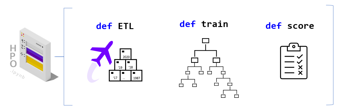
As we’ve already mentioned, the SageMaker Estimator represents the containerized software stack that AWS SageMaker will replicate to each worker node.

The first step to building our Estimator, is to augment a RAPIDS container with our ML Workflow code from above, and push this image to Amazon Elastic Cloud Registry so it is available to SageMaker.

2.1 - Containerize and Push to ECR

Now let’s turn to building our container so that it can integrate with the AWS SageMaker HPO API.

Our container can either be built on top of the latest RAPIDS [ nightly ] image as a starting layer or the RAPIDS stable image.

rapids_stable = "rapidsai/rapidsai:21.06-cuda11.0-base-ubuntu18.04-py3.7"
rapids_nightly = "rapidsai/rapidsai-nightly:21.08-cuda11.0-base-ubuntu18.04-py3.7"

rapids_base_container = rapids_stable
assert rapids_base_container in [rapids_stable, rapids_nightly]

Let’s also decide on the full name of our container.

image_base = "cloud-ml-sagemaker"
image_tag = rapids_base_container.split(":")[1]

ecr_fullname = f"{account[0]}.dkr.ecr.{region[0]}.amazonaws.com/{image_base}:{image_tag}"

ecr_fullname

2.1.1 - Write Dockerfile

We write out the Dockerfile to disk, and in a few cells execute the docker build command.

Let’s now write our selected RAPDIS image layer as the first FROM statement in the the Dockerfile.

with open("Dockerfile", "w") as dockerfile:
    dockerfile.writelines(
        f"FROM {rapids_base_container} \n\n"
        f'ENV DATASET_DIRECTORY="{dataset_directory}"\n'
        f'ENV ALGORITHM_CHOICE="{algorithm_choice}"\n'
        f'ENV ML_WORKFLOW_CHOICE="{ml_workflow_choice}"\n'
        f'ENV CV_FOLDS="{cv_folds}"\n'
    )

Next let’s append write the remaining pieces of the Dockerfile, namely adding the sagemaker-training-toolkit, flask, dask-ml, and copying our python code.

%%writefile -a Dockerfile

# ensure printed output/log-messages retain correct order
ENV PYTHONUNBUFFERED=True

# delete expired nvidia keys and fetch new ones
RUN apt-key del 7fa2af80
RUN rm /etc/apt/sources.list.d/cuda.list
RUN rm /etc/apt/sources.list.d/nvidia-ml.list
RUN wget https://developer.download.nvidia.com/compute/cuda/repos/ubuntu1804/x86_64/cuda-keyring_1.0-1_all.deb && dpkg -i cuda-keyring_1.0-1_all.deb

# add sagemaker-training-toolkit [ requires build tools ], flask [ serving ], and dask-ml
RUN apt-get update && apt-get install -y --no-install-recommends build-essential \
    && source activate rapids && pip3 install sagemaker-training dask-ml flask

# path where SageMaker looks for code when container runs in the cloud
ENV CLOUD_PATH "/opt/ml/code"

# copy our latest [local] code into the container
COPY . $CLOUD_PATH

# make the entrypoint script executable
RUN chmod +x $CLOUD_PATH/entrypoint.sh

WORKDIR $CLOUD_PATH
ENTRYPOINT ["./entrypoint.sh"]

Lastly, let’s ensure that our Dockerfile correctly captured our base image selection.

validate_dockerfile(rapids_base_container)
!cat Dockerfile

2.1.2 Build and Tag

The build step will be dominated by the download of the RAPIDS image (base layer). If it’s already been downloaded the build will take less than 1 minute.

!docker pull $rapids_base_container

%%time
!docker build . -t $ecr_fullname -f Dockerfile

2.1.3 - Publish to Elastic Cloud Registry (ECR)

Now that we’ve built and tagged our container its time to push it to Amazon’s container registry (ECR). Once in ECR, AWS SageMaker will be able to leverage our image to build Estimators and run experiments.

Docker Login to ECR

docker_login_str = !(aws ecr get-login --region {region[0]} --no-include-email)

!{docker_login_str[0]}

Create ECR repository [ if it doesn’t already exist]

repository_query = !(aws ecr describe-repositories --repository-names $image_base)
if repository_query[0] == '':
    !(aws ecr create-repository --repository-name $image_base)

Let’s now actually push the container to ECR > Note the first push to ECR may take some time (hopefully less than 10 minutes).

!docker push $ecr_fullname

2.2 - Create Estimator

Having built our container [ +custom logic] and pushed it to ECR, we can finally compile all of efforts into an Estimator instance.

# 'volume_size' - EBS volume size in GB, default = 30
estimator_params = {
    "image_uri": ecr_fullname,
    "role": execution_role,
    "instance_type": instance_type,
    "instance_count": 1,
    "input_mode": "File",
    "output_path": s3_model_output,
    "use_spot_instances": use_spot_instances_flag,
    "max_run": max_duration_of_experiment_seconds,  # 24 hours
    "sagemaker_session": session,
}

if use_spot_instances_flag == True:
    estimator_params.update({"max_wait": max_duration_of_experiment_seconds + 1})

estimator = sagemaker.estimator.Estimator(**estimator_params)

2.3 - Test Estimator

Now we are ready to test by asking SageMaker to run the BYOContainer logic inside our Estimator. This is a useful step if you’ve made changes to your custom logic and are interested in making sure everything works before launching a large HPO search.

Note: This verification step will use the default hyperparameter values declared in our custom train code, as SageMaker HPO will not be orchestrating a search for this single run.

summarize_choices(
    s3_data_input,
    s3_model_output,
    ml_workflow_choice,
    algorithm_choice,
    cv_folds,
    instance_type,
    use_spot_instances_flag,
    search_strategy,
    max_jobs,
    max_parallel_jobs,
    max_duration_of_experiment_seconds,
)

job_name = new_job_name_from_config(
    dataset_directory, region, ml_workflow_choice, algorithm_choice, cv_folds, instance_type
)

estimator.fit(inputs=s3_data_input, job_name=job_name.lower())

3. Run HPO

With a working SageMaker Estimator in hand, the hardest part is behind us. In the key choices section we already defined our search strategy and hyperparameter ranges, so all that remains is to choose a metric to evaluate performance on. For more documentation check out the AWS SageMaker Hyperparameter Tuner documentation.

3.1 - Define Metric

We only focus on a single metric, which we call ‘final-score’, that captures the accuracy of our model on the test data unseen during training. You are of course welcome to add aditional metrics, see AWS SageMaker documentation on Metrics. When defining a metric we provide a regular expression (i.e., string parsing rule) to extract the key metric from the output of each Estimator/worker.

metric_definitions = [{"Name": "final-score", "Regex": "final-score: (.*);"}]

objective_metric_name = "final-score"

3.2 - Define Tuner

Finally we put all of the elements we’ve been building up together into a HyperparameterTuner declaration.

hpo = sagemaker.tuner.HyperparameterTuner(
    estimator=estimator,
    metric_definitions=metric_definitions,
    objective_metric_name=objective_metric_name,
    objective_type="Maximize",
    hyperparameter_ranges=hyperparameter_ranges,
    strategy=search_strategy,
    max_jobs=max_jobs,
    max_parallel_jobs=max_parallel_jobs,
)

3.3 - Run HPO

summarize_choices(
    s3_data_input,
    s3_model_output,
    ml_workflow_choice,
    algorithm_choice,
    cv_folds,
    instance_type,
    use_spot_instances_flag,
    search_strategy,
    max_jobs,
    max_parallel_jobs,
    max_duration_of_experiment_seconds,
)

Let’s be sure we take a moment to confirm before launching all of our HPO experiments. Depending on your configuration options running this cell can kick off a massive amount of computation! > Once this process begins, we recommend that you use the SageMaker UI to keep track of the health of the HPO process and the individual workers.

tuning_job_name = new_job_name_from_config(
    dataset_directory, region, ml_workflow_choice, algorithm_choice, cv_folds, instance_type
)
hpo.fit(inputs=s3_data_input, job_name=tuning_job_name, wait=True, logs="All")

hpo.wait()  # block until the .fit call above is completed

3.4 - Results and Summary

Once your job is complete there are multiple ways to analyze the results. Below we display the performance of the best job, as well printing each HPO trial/job as a row of a dataframe.

hpo_results = summarize_hpo_results(tuning_job_name)

sagemaker.HyperparameterTuningJobAnalytics(tuning_job_name).dataframe()

For a more in depth look at the HPO process we invite you to check out the HPO_Analyze_TuningJob_Results.ipynb notebook which shows how we can explore interesting things like the impact of each individual hyperparameter on the performance metric.

3.5 - Getting the best Model

Next let’s download the best trained model from our HPO runs.

local_filename, s3_path_to_best_model = download_best_model(
    model_output_bucket, s3_model_output, hpo_results, best_hpo_model_local_save_directory
)

3.6 - Model Serving

With your best model in hand, you can now move on to serving this model on SageMaker.

In the example below we show you how to build a RealTimePredictor using the best model found during the HPO search. We will add a lightweight Flask server to our RAPIDS Estimator (a.k.a., container) which will handle the incoming requests and pass them along to the trained model for inference. If you are curious about how this works under the hood check out the Use Your Own Inference Server documentation and reference the code in code/serve.py.

If you are interested in additional serving options (e.g., large batch with batch-transform), we plan to add a companion notebook that will provide additional details.

3.6.1 - GPU serving

endpoint_model = sagemaker.model.Model(
    image_uri=ecr_fullname, role=execution_role, model_data=s3_path_to_best_model
)

DEMO_SERVING_FLAG = False

if DEMO_SERVING_FLAG:
    endpoint_model.deploy(initial_instance_count=1, instance_type="ml.p3.2xlarge")

if DEMO_SERVING_FLAG:

    predictor = sagemaker.predictor.Predictor(
        endpoint_name=str(endpoint_model.endpoint_name), sagemaker_session=session
    )
    """ Below we've compiled examples to sanity test the trained model performance on the Airline dataset.
        The first is from a real flight that was nine minutes early in departing,
        the second example is from a flight that was 123 minutes late in departing.
    """
    if dataset_directory in ["1_year", "3_year", "10_year"]:
        on_time_example = [
            2019.0,
            4.0,
            12.0,
            2.0,
            3647.0,
            20452.0,
            30977.0,
            33244.0,
            1943.0,
            -9.0,
            0.0,
            75.0,
            491.0,
        ]
        late_example = [
            2018.0,
            3.0,
            9.0,
            5.0,
            2279.0,
            20409.0,
            30721.0,
            31703.0,
            733.0,
            123.0,
            1.0,
            61.0,
            200.0,
        ]
        example_payload = str(list([on_time_example, late_example]))
    else:
        example_payload = ""  # fill in a sample payload

    print(example_payload)
    predictor.predict(example_payload)

Once we are finished with the serving example, we should be sure to clean up and delete the endpoint.

if DEMO_SERVING_FLAG:

    predictor.delete_endpoint()

Summary

We’ve now successfully built a RAPIDS ML workflow, containerized it (as a SageMaker Estimator), and launched a set of HPO experiments to find the best hyperparamters for our model.

If you are curious to go further, we invite you to plug in your own dataset and tweak the configuration settings to find your champion model!

HPO Experiment Details

As mentioned in the introduction we find a 12X speedup in wall clock time and a 4.5x reduction in cost when comparing between GPU and CPU instances on 100 HPO trials using 10 parallel workers on 10 years of the Airline Dataset (~63M flights). In these experiments we used the XGBoost algorithm with the multi-GPU vs multi-CPU Dask cluster and 10 cross validaiton folds. Below we offer a table with additional details.

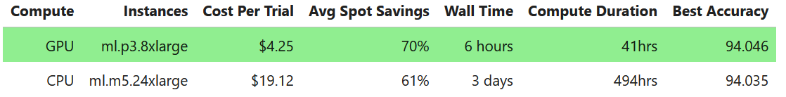
In the case of the CPU runs, 12 jobs were stopped since they exceeded the 24 hour limit we set. CPU Job Summary Image

In the case of the GPU runs, no jobs were stopped. GPU Job Summary Image

Note that in both cases 1 job failed because a spot instance was terminated. But 1 failed job out of 100 is a minimal tradeoff for the significant cost savings.

Appendix: Bring Your Own Dataset Checklist

If you plan to use your own dataset (BYOD) here is a checklist to help you integrate into the workflow:

• ☐ Dataset should be in either CSV or Parquet format.

• ☐ Dataset is already pre-processed (and all feature-engineering is done).

• ☐ Dataset is uploaded to S3 and data_bucket and dataset_directory have been set to the location of your data.

• ☐ Dataset feature and target columns have been enumerated in /code/HPODataset.py

Rapids References

cloud-ml-examples

RAPIDS HPO

cuML Documentation

SageMaker References

SageMaker Training Toolkit

Estimator Parameters

Spot Instances docs, and `blog <>`__

Notebook CI Test Results

This notebook was tested in multiple regions. The test results are as follows, except for us-west-2 which is shown at the top of the notebook.