Supplement your data with synthetic features from a pre-trained model to train a better downstream audio classification model
This notebook’s CI test result for us-west-2 is as follows. CI test results in other regions can be found at the end of the notebook.
Training models on real life audio datasets can be challenging. Often, these datasets have noise from the environment that distorts the signal in the audio and this can affect the quality of the models that are trained on such datasets. Cleaning the dataset using traditional methods like filtering based on signal’s characteristics like spectral energy, amplitude, frequency, etc is complicated and consumes a lot of time that often involves a lot of trial and error.
Sometimes machine learning models that are trained to identify and separate the different components (like background and foreground, vocals and accompaniment) in an audio file can be used to generate synthetic features or to clean the original audio dataset. The Quantiphi Source Separation Model is one such model that performs source separation in the time domain of the input source audio. It uses a convolutional neural network like a U-Net in the time domain to separate the background noise and the main signal in an input audio.
In this sample notebook, you will see how to use this model to process original audio files and then use the output of the model to train other downstream models. The performance of the downstream models is often better than one that has been trained on the original audio data.
Overview:
Industrial machinery is often categorized as critical equipment in manufacturing processes. This equipment is prone to failure or breakdown, resulting in significant expenses for companies. There is a lot of value in monitoring these machines using different sensors including microphones. Advancements in acoustic detection methods as well as algorithms that aid in classification of scenes and events can now be used to monitor them. In this notebook, you will use an existing dataset of industrial machine sounds that contains sounds of normal and malfunctioning industrial machines.
The methodology can be applied to various real-life scenarios where anomalous sounds are recorded (e.g., contamination, leakage, rotating unbalance, and rail damage). The purpose of this notebook is to use a pre-trained machine learning model and show if it can contribute to achieve better performance in acoustic classification based models.
In step 1 of this notebook, you will download the dataset that is used in the notebook. In step 2, you will create the model from an AWS Marketplace subscription, deploy to an Amazon SageMaker endpoint and use it to preprocess the original audio files. In step 3, you will explore the output of the model and see some examples. In step 4, you will build classification models to identify anomalous samples. In Step 5 you will compare the performance of the models.
Contents:
Usage instructions
You can run this notebook one cell at a time (By using Shift+Enter for running a cell).
Prerequisites
This notebook requires the IAM role associated with this notebook to have AmazonSageMakerFullAccess IAM permission.
Pick instance type ‘ml.t3.large’ or larger. Set kernel to ‘conda_python3’ in a SageMaker Notebook instance and to ‘Python 3 Data Science’ in SageMaker Studio.
This sample notebook requires a subscription to Source Separation by Quantiphi, a pre-trained machine learning model package from AWS Marketplace. If your AWS account has not been subscribed to this listing, here is the process you can follow:
Open the listing from AWS Marketplace.
Read the Highlights section and then product overview section of the listing.
View usage information and then additional resources.
Note the supported instance types.
Next, click on Continue to subscribe.
Review End-user license agreement, support terms, as well as pricing information.
“Accept Offer” button needs to be clicked if your organization agrees with EULA, pricing information as well as support terms. If Continue to configuration button is active, it means your account already has a subscription to this listing. Once you click on Continue to configuration button and then choose region, you will see that a Product ARN will appear. Specify the value in the following cell.
The below ARN is the version on which the notebook was tested. Please use this as a fallback if a newer version does not work. Additionally, you can refer this file for a list of ARNs corresponding to different regions.
[ ]:
# This is the ARN obtained in the above step
model_package_arn = "arn:aws:sagemaker:us-east-2:057799348421:model-package/source-sep11618586387-e73722215b88850c22e59b7564075da5"
Installing Dependencies
Install the librosa package. This is a useful python library for audio analysis.
[ ]:
# Install librosa for audio analysis
!conda install -y -c conda-forge librosa
[ ]:
import glob
import pandas as pd
import sagemaker as sm
import zipfile
import os
import shutil
import json
import uuid
import librosa
import librosa.display
import soundfile as sf
import boto3
import numpy as np
import matplotlib.pyplot as plt
from sklearn.model_selection import train_test_split
from sklearn.ensemble import GradientBoostingClassifier
from sklearn.model_selection import RandomizedSearchCV
from sklearn.metrics import (
    confusion_matrix,
    f1_score,
    recall_score,
    precision_score,
    plot_confusion_matrix,
    fbeta_score,
)
from sagemaker import ModelPackage
from IPython.display import Audio
[ ]:
role = sm.get_execution_role()
sagemaker_session = sm.Session()
s3 = boto3.resource("s3")
Step 1: Data collection and preparation
In this notebook, you will apply the above idea to the Malfunctioning Industrial Machine Investigation and Inspection (MIMII) dataset. This dataset consists of normal and anomalous sounds of industrial machines like pumps, fans, valves and slide rails. The goal is to train a model to identify the anomalous sounds.
The notebook uses the ‘pump’ dataset and you can experiment with other datasets in the family as an exercise. This consists of 4 different kinds (models) of pumps. Overall, there are around 3700 ‘normal’ samples and around 450 ‘anomalous’ samples. These have been split into ‘train’ and ‘test’, with ‘train’ consisting of only ‘normal’ samples. Since you will be building a classification model to identify anomalous samples, all the audio files are merged and then randomly split to a training and test set in a stratified fashion.
Step 1.1: Download the dataset
The first step is to download the dataset from its source and unzip the contents into a directory.
[ ]:
os.environ["RAW_DATA"] = "DEMO-midii-audio"
os.environ["RAW_DATA_PUMP"] = "DEMO-midii-audio/pump"
[ ]:
!wget -O dev_data_pump.zip https://zenodo.org/record/3678171/files/dev_data_pump.zip?download=1
!rm -rf $RAW_DATA
!mkdir $RAW_DATA
!unzip dev_data_pump.zip -d $RAW_DATA/
!rm dev_data_pump.zip
Let’s also create a dataframe to store the details of each audio sample in the dataset, and the location of the source file.
[ ]:
# Get a list of files that have been downloaded across the different folders
# data/pump
# ________/train/
# ________/test/
dirs = glob.glob(os.environ["RAW_DATA_PUMP"] + "/*/*")

samples = []

# Parse through the list and record metadata about the sample
for idx, path in enumerate(dirs):
    samples.append(
        (
            idx,
            path.split("/")[1],
            path.split("/")[2],
            path.split("/")[3].split("_")[0],
            path.split("/")[3].split("_")[1] + path.split("/")[3].split("_")[2],
            path,
        )
    )
audio_samples = pd.DataFrame(
    samples, columns=["ID", "machine", "set", "sample_type", "model", "file_path"]
)

# Move all the files into a single folder - data/pump
samples = []
for i, row in audio_samples.iterrows():
    destination = "%s/%s_%s" % (
        os.environ["RAW_DATA_PUMP"],
        row["set"],
        row["file_path"].split("/")[-1],
    )
    shutil.move(row["file_path"], destination)
    row["file_path"] = destination
    samples.append(row)
audio_samples = pd.DataFrame(
    samples, columns=["ID", "machine", "model", "sample_type", "file_path"]
)
[ ]:
!rm -r $RAW_DATA_PUMP/train $RAW_DATA_PUMP/test
[ ]:
!du -sh $RAW_DATA/pump
Step 1.2: Upload the input data to s3 bucket
Next, you will create a folder and copy all the audio files into this folder in an s3 bucket.
The size of the dataset is around 1.3G and since you are uploading such a large dataset, the following step takes around 3-4 minutes.
[ ]:
bucket = sagemaker_session.default_bucket()
[ ]:
# Upload all the orignal files to s3

transform_input = sagemaker_session.upload_data(
    os.environ["RAW_DATA_PUMP"], bucket=bucket, key_prefix="pump"
)  # no trailing '/'
print("Transform input uploaded to " + transform_input)
Step 2: Use an ML model to clean the audio data
You will now use the Quantiphi source-separation model that was introduced earlier in the notebook. The prediction is in the form of two audio files comprising of the vocals and accompaniment (signal/noise). The output is a zipped folder containing the above two audio files.
Step 2.1: Specify model arn from AWS Marketplace subscription and create model from model package
You will use ModelPackageArnProvider class to make sure you get the correct ARN in every supported region and then use the ModelPackage class to create the model.
[ ]:
print("Using model package ARN to create a dynamic model - " + model_package_arn)

model = ModelPackage(
    role=role, model_package_arn=model_package_arn, sagemaker_session=sagemaker_session
)
Step 2.2: Run a batch transform job
Finally you will run a batch transform job to process all the audio files using the model declared in the earlier step.
You are also going to specify an instance type for the batch transformation. You can refer to compatible instance types for this AWS Marketplace offering.
This step takes around 30 minutes or more with the parameters that are used. You may increase the ‘instance_count’ to increase the speed. You can also explore changing the ‘instance_type’ to a more powerful instance.
[ ]:
# Define a variable that is used as a prefix to create a folder in the s3 bucket.
prefix = "pump-source-separated/"
Create a folder in the S3 bucket. The S3 URI of this folder is passed as the ‘output_path’ in the next step.
[ ]:
source_separated_output = sagemaker_session.upload_string_as_file_body(
    body="", bucket=bucket, key=prefix
)
[ ]:
# run a batch transform job to score all the audio files
transformer = model.transformer(
    instance_count=32,
    instance_type="ml.m4.2xlarge",
    strategy="SingleRecord",
    output_path=source_separated_output,
)
transformer.transform(transform_input, content_type="application/x-recordio-protobuf")
transformer.wait()

print("Batch Transform output saved to " + transformer.output_path)
Step 2.3: Download the output of the batch transform job
You will now download the output from the batch transform job. The model outputs a single zip for every audio file in the input. The zip contains two files, a vocals file and an accompaniment file.
Create a folder to store the downloaded data.
[ ]:
os.environ["SOURCE_SEPARATED_DATA"] = os.environ["RAW_DATA"] + "/pump-source-separated/"
[ ]:
!rm -rf $SOURCE_SEPARATED_DATA
!mkdir $SOURCE_SEPARATED_DATA
Download the files from the s3 bucket.
[ ]:
my_bucket = s3.Bucket(bucket)
count = 0

# Download the .zip files(output from the source separation model) from the s3 bucket
for object_summary in my_bucket.objects.filter(Prefix=prefix):
    count += 1
    file_name = object_summary.key.split("/")[-1]

    if file_name == prefix.split("/")[-1]:
        continue
    # print(prefix+file_name)
    my_bucket.download_file(
        object_summary.key, "{}/{}.zip".format(os.environ["SOURCE_SEPARATED_DATA"], file_name)
    )
Unzip all the downloaded files. You will find that every folder has two files: ’*_accompaniment.wav’ and ’*_vocals.wav’. These are the new source-separated audio files.
[ ]:
!find $SOURCE_SEPARATED_DATA -name '*.zip' -exec sh -c 'unzip -d "${1%.*}" "$1"' _ {} \;
Step 3: Explore the source separated audio files
You can use the below function to explore the output of the source separation model. This is done in the next step.
The function loads the audio file using the librosa package and plots them using the ‘waveplot’ function from the library. The input to the function is the path to the original audio sample. The function plots that and then loads the corresponding source-separated files for plotting.
[ ]:
def plot_waveform(file):
    """
    Function to plot the waveform of the original sample and the corresponding source-separated signals

    file: path of a original audio sample

    """
    print("--- Original Audio sample ---")
    display(Audio(file))

    # Load the original audio file and plot the amplitude of the signal
    x, sr = librosa.load(file, sr=16000, mono=False)
    librosa.display.waveplot(x, sr, label="original audio")
    plt.legend()
    plt.title("Original Audio - waveplot")
    plt.show()

    # Find the corresponding source separated files for the original audio file selected above
    file_id = file.split("/")[-1]
    accompaniment_file = glob.glob(
        f'{os.environ["SOURCE_SEPARATED_DATA"]}/{file_id}.out/output/*_accompaniment.wav'
    )
    vocal_file = glob.glob(
        f'{os.environ["SOURCE_SEPARATED_DATA"]}/{file_id}.out/output/*_vocals.wav'
    )

    print("--- Source separated: Accompaniment ---")
    display(Audio(accompaniment_file[0]))
    print("--- Source separated: Vocal ---")
    display(Audio(vocal_file[0]))

    # Load the accompaniment and vocal file and plot the amplitudes of the two waveforms
    x, sr = librosa.load(accompaniment_file[0], sr=16000, mono=False)
    librosa.display.waveplot(x, sr, color="grey", label="accompaniment")

    x, sr = librosa.load(vocal_file[0], sr=16000, mono=False)
    librosa.display.waveplot(x, sr, color="teal", alpha=0.8, label="vocals")
    plt.legend()
    plt.title("Source Separated Audio - waveplots")
    plt.show()
Plot the waveform of an anomalous sample and the corresponding source-separated audio files. Note the difference in the waveforms. The source-separation model has separated the original into two distinct signals.
For the purpose of illustration, a specific example is selected. You can modify the input to ‘plot_waveform’ and take a look at other samples of your choice.
[ ]:
plot_waveform(os.environ["RAW_DATA_PUMP"] + "/test_anomaly_id_00_00000133.wav")
In this example, you look at a normal sample. The ‘vocals’ file has a signal with a much smaller amplitude than the original audio except towards the very end. While the ‘accompaniment’ more or less retains the properties of the original audio file.
[ ]:
plot_waveform(os.environ["RAW_DATA_PUMP"] + "/train_normal_id_00_00000131.wav")
Step 4: Build a classification model to identify anomalous samples
The next step is to build a classification model to identify those samples that are anomalous. Since the primary goal of this notebook is to demonstrate the effectiveness of using a pre-trained model to clean the audio data, this notebook uses a Gradient Boosting Classifier. You can however try other approaches such as convolutional neural networks, autoencoders, etc.
You will train a Gradient Boosting Classifier using the raw audio files and the source separated audio files respectively, and then compare the performance of models on the test data.
Step 4.1: Introduction to Audio Feature Extraction
An audio file or a signal is generally a sequence of samples at a particular “sampling” frequency and a “sampling” resolution. The audio files in the MIMII dataset have a sampling frequency of 16kHz.
The first step to build a model on audio data is to convert the original audio signal into a higher representation that captures all its properties. This is done by splitting the input signal into short term windows and extracting features from it.
There are different kinds of features that can be extracted: - Time domain features: These are directly extracted from the audio sample. - Frequency domain features: These features are extracted from the Discrete Fourier Transform of the audio signal. - Cepstral features: These features are obtained by applying the Inverse Fourier Transform of the logarithm of the estimated signal.
Optional reading
You can learn more about the different kinds of features and the various libraries that can be used to compute them in this paper.
Step 4.2: Compute Mel-frequency cepstral coefficients (MFCCs)
You will use a well known python library for audio analysis called librosa to compute Mel-frequency cepstral coefficients (MFCCs). These fall into the category of cepstral features.
MFCCs are computed for every window (or frame) in the audio signal. Hence, you will compute a statistic to aggregate this over all the windows in the audio signal. In this case, the mean is computed. However, you can compute different percentiles and use them as features.
You are going to do the following in this step: - Compute MFCCs for every audio sample in the dataset (i.e. for both the raw audio file and the source separated files - accompaniment.wav and vocals.wav). - Compute the mean of the MFCCs across the different windows. - Record the label of the audio sample. Anomalous samples are considered as ‘positive’ samples (class = 1).
[ ]:
mfcc_raw = []
mfcc_accompaniment = []
mfcc_vocal = []
labels = []

# set the sampling rate equal to that defined in the dataset
sampling_rate = 16000

# set the number of MFCCs that you want to use.
# There are 128 of them and you should use all of them
num_mfccs = 128

for i, row in audio_samples.iterrows():

    # raw audio
    x, rate = librosa.load(row["file_path"], sr=sampling_rate)
    features = np.mean(librosa.feature.mfcc(x, sr=rate, n_mfcc=num_mfccs), axis=1)
    mfcc_raw.append(features)

    file_id = row["file_path"].split("/")[-1]
    accompaniment_file = glob.glob(
        f'{os.environ["SOURCE_SEPARATED_DATA"]}/{file_id}.out/output/*_accompaniment.wav'
    )
    vocal_file = glob.glob(
        f'{os.environ["SOURCE_SEPARATED_DATA"]}/{file_id}.out/output/*_vocals.wav'
    )

    # accompaniment
    x, rate = librosa.load(accompaniment_file[0])
    features = np.mean(librosa.feature.mfcc(x, sr=rate, n_mfcc=num_mfccs), axis=1)
    mfcc_accompaniment.append(features)

    # vocals
    x, rate = librosa.load(vocal_file[0])
    features = np.mean(librosa.feature.mfcc(x, sr=rate, n_mfcc=num_mfccs), axis=1)
    mfcc_vocal.append(features)

    labels.append(1 if row["sample_type"] == "anomaly" else 0)
To make it easy to access the features, you will now concatenate all the features into a single dataframe and name the columns appropriately.
[ ]:
# Concatenate dataframes into a single pandas dataframe.
mfcc_features = pd.concat(
    [
        pd.DataFrame(mfcc_raw, columns=[f"mfcc_{i}_raw" for i in range(mfcc_raw[0].shape[0])]),
        pd.DataFrame(
            mfcc_accompaniment,
            columns=[f"mfcc_{i}_accompaniment" for i in range(mfcc_accompaniment[0].shape[0])],
        ),
        pd.DataFrame(mfcc_raw, columns=[f"mfcc_{i}_vocals" for i in range(mfcc_vocal[0].shape[0])]),
    ],
    axis=1,
)

# store the column names for the features from the raw(original) audio
mfcc_raw = [col for col in mfcc_features.columns if col.endswith("raw")]

# store the column names for the features from the source separated files: accompaniment and vocal
mfcc_accompaniment = [col for col in mfcc_features.columns if col.endswith("accompaniment")]
mfcc_vocals = [col for col in mfcc_features.columns if col.endswith("vocals")]
Step 4.3: Split the samples into ‘training’ and ‘test’ datasets.
You will now create a ‘training’ and a ‘test’ dataset by splitting all the samples in a stratified fashion. Use ‘test_size’ to decide the percentage of samples in your test data (20% in this case). Stratification is done by passing the labels as an argument to ‘stratify’. This ensures that the split is done such that the proportion of anomalous samples is the same in the training and test datasets.
[ ]:
X_train, X_test, y_train, y_test = train_test_split(
    mfcc_features, labels, test_size=0.2, shuffle=True, stratify=labels, random_state=1
)
Step 4.4: Train a classifier on the raw audio data.
The hyperparameters of the model have been set to reasonable defaults. The number of trees is set to 1000 and the sampling fraction is 0.5. This ensures that variance is reduced. The same hyperparameters are used in all the models for consistency during comparison.
[ ]:
# Train a GradientBoosting Classifier from sklearn. In a production setting, you can use xgboost, lightgbm, etc.
clf_raw = GradientBoostingClassifier(
    subsample=0.5, n_estimators=1000, max_features="log2", random_state=10
)
clf_raw.fit(X_train[mfcc_raw], y_train)
y_pred_raw = clf_raw.predict(X_test[mfcc_raw])
Step 4.5: Train a classifier on the ‘source-separated’ audio data.
In this step, you will train two ML models, one on vocals and another one on accompaniment.
[ ]:
# Train a GradientBoosting Classifier using only the features from 'accompaniment'
clf_accompaniment = GradientBoostingClassifier(
    subsample=0.5, n_estimators=1000, max_features="log2", random_state=10
)
clf_accompaniment.fit(X_train[mfcc_accompaniment], y_train)
y_pred_accompaniment = clf_accompaniment.predict(X_test[mfcc_accompaniment])

# Train a GradientBoosting Classifier using only the features from 'vocals'
clf_vocals = GradientBoostingClassifier(
    subsample=0.5, n_estimators=1000, max_features="log2", random_state=10
)
clf_vocals.fit(X_train[mfcc_vocals], y_train)
y_pred_vocals = clf_vocals.predict(X_test[mfcc_vocals])
Step 5: Performance Comparison
After training the models, it is time to compare their performance. You will now compute the accuracy, recall, and f2-score on the ‘test’ dataset.
Since this is a binary classification problem with imbalanced classes, recall, and the f2-score are the metrics of importance.
F2-score is a variation of the F-measure that weights recall higher than precision.
In this specific scenario, the goal is to identify pumps that are not functioning properly (anomalous) using their sound. The cost of not identifying anomalous pumps is greater for the business. This makes Recall and F2-score the metrics that we should optimize since they capture the extent to which the positive class is correctly predicted. In this case, it’s the anomalous class.
Step 5.1: Compute Accuracy, Recall and F2-Score
In this step, you will compute the Recall and F2 Score on the test data using the different models that were trained in the previous step. You will also plot the confusion matrix.
[ ]:
print("----------------- Original Audio Data ---------------------")
print("Recall: %.2f" % (recall_score(y_test, y_pred_raw)))
print("F2 Score: %.2f" % (fbeta_score(y_test, y_pred_raw, beta=2.0)))
plot_confusion_matrix(clf_raw, X_test[mfcc_raw], y_test)
plt.show()

print("----------------- Source-separated: Accompaniment ---------------------")
print("Recall: %.2f" % (recall_score(y_test, y_pred_accompaniment)))
print("F2 Score: %.2f" % (fbeta_score(y_test, y_pred_accompaniment, beta=2.0)))
plot_confusion_matrix(clf_accompaniment, X_test[mfcc_accompaniment], y_test)
plt.show()

print("----------------- Source-separated: Vocals ---------------------")
print("Recall: %.2f" % (recall_score(y_test, y_pred_vocals)))
print("F2 Score: %.2f" % (fbeta_score(y_test, y_pred_vocals, beta=2.0)))
plot_confusion_matrix(clf_vocals, X_test[mfcc_vocals], y_test)
plt.show()
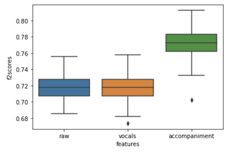
Results
From the above results, it is clear that a model that is trained on the output of the source separation model performs better than one trained on the original audio data.
The ‘F2-Score’ and ‘Recall’ of the model trained on the ‘accompaniment audio signal’ which is the output of the source separation model is greater than that of the model trained with the original audio. This implies that the model correctly identifies more anomalous signals and is hence better.
The metrics that you see might slightly vary because these are tree based models and have a certain level of randomness associated with it. However, we did run the model multiple times and found that the model trained on the ‘accompaniment audio files’ generally gives a 5% - 10% higher F2 score.
Step 6: Conclusion and next steps
In this notebook, you have done the following - - used a Machine Learning model to create synthetic features and preprocess the audio data - showed that training a downstream model on the processed data can enhance its performance
In terms of the business value of the problem we see more and more use cases around sound-based predictive maintenance and it is considered as the future of predictive maintenance. A majority of the machine components produce sounds and hence these signals can be captured to monitor them.
Techniques above show how to improve the models quickly and efficiently using pre-trained models from collective intelligence across industries.
SageMaker Marketplace has various similar pre-trained models for other tasks that can increase model accuracy in current models using existing models.
Step 6.1: Cancel AWS Marketplace subscription
Finally, if you subscribed to AWS Marketplace model for an experiment and would like to unsubscribe, you can follow the steps below. Before you cancel the subscription, ensure that you do not have any deployable model created from the model package or using the algorithm. You can also find this information by looking at the container name associated with the model. In this case, the name follows the following pattern - ‘source-sepxxxxxx’.
Steps to unsubscribe from the product on AWS Marketplace:
Navigate to Machine Learning tab on your Software subscriptions page. Locate the listing that you would need to cancel, and click Cancel Subscription.
This notebook was tested in multiple regions. The test results are as follows, except for us-west-2 which is shown at the top of the notebook.